Contents · 9 sections
1What problem is it solving?2Does filtering first change the recommendations?3The pipeline4Why slice the index by decoding step?5Why fewer scores are not automatically faster6Does it actually work better?7Limitations as I see them8How a recommendation team could try it9VerdictSHARE

Engineering teams serving generative recommenders should read this: it shows that most constrained-decoding compute goes to candidates that will be discarded, and gives a full filter-first system implementation. Generative recommenders emit item codes one token at a time, and every step must keep the code pointing at an item that really exists in the catalog. The usual approach scores every possible next token and then filters out the invalid ones, but most combinations are invalid anyway, so those scores are wasted. The authors first check whether the order can be flipped: filtering before scoring returns about 99.9% of the same items, with almost no change in quality. ZeroGR does two things around this order. First, it slices the filtering index by decoding step, stored sparsely when a step has few valid candidates and densely when it has many, which saves GPU memory. Second, it changes how the work runs on the GPU: each prefix gets fixed candidate slots, and for each step a measurement made in advance picks full scoring or scoring only valid tokens. This is what turns fewer scores into a real speedup. Against representative baselines, the combined filtering, scoring and candidate selection stage runs up to 9.9 times faster.
What problem is it solving?
Generative recommenders generate an item's SID step by step with beam search, and similar items share the first SID tokens. At each step the model scores the next token for every beam. But the SID space is huge: in production, all possible combinations far exceed 10^16, while only ten million to a hundred million correspond to real items. So each step must also filter, keeping only tokens that can still lead to a real item.
An illustrative example: only two items in the catalog have SIDs starting with 3-5, namely 3-5-1 and 3-5-4. Once a beam has generated 3-5, the only valid next tokens are 1 and 4.
| Approach (illustrative) | Scores computed for this beam at step 3 | Kept |
|---|---|---|
| Score, then filter | every token allowed at this position (the codebook), say 2,048 | 2 |
| Filter, then score | only tokens 1 and 4 | 2 |
Scoring first runs one large matrix product over all tokens and then masks out the invalid ones. The later the step, the fewer valid tokens remain, and the larger the wasted share.
Does filtering first change the recommendations?
The two orders are not exactly equivalent. Scores go through a softmax: when scoring first, the denominator covers all tokens; when filtering first, only valid tokens. If a prefix puts noticeable probability on invalid tokens, filtering first boosts its valid candidates more, which can change which beams survive.
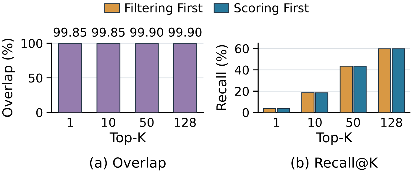
The authors test this with a generative recommender trained on MovieLens-1M. The two orders return lists that overlap 99.85% to 99.90%, with nearly identical Recall at every cutoff. The reason lies in how decoding narrows: in early steps many tokens are still valid and a trained model already puts almost all probability on them, so dropping invalid tokens barely changes the denominator; in later steps few tokens are valid, but a candidate's total score comes mostly from earlier steps, so the order rarely changes which candidates are kept. Unchanged quality is the precondition for filtering first.
The pipeline
ZeroGR has three parts: a filtering index built offline, an execution engine that uses it at every decoding step, and a pipeline that rebuilds the index when the model is updated. Each online step has four stages. First, the model outputs each beam's hidden vector. Second, the index returns the beam's valid tokens. Third, the valid tokens are scored: steps with few candidates score only valid tokens, while steps with many score everything and then pick out the valid ones. Fourth, a log-softmax runs over the valid tokens only, the resulting log-probability is added to the beam's accumulated log-probability, and the next beams are selected by this new total.
Why slice the index by decoding step?
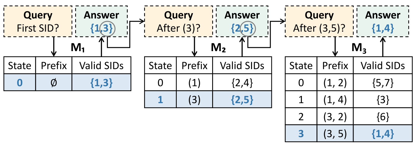
The obvious index is a prefix tree. But at step 3, decoding only asks what can follow a length-2 prefix; it never needs the whole tree. So ZeroGR splits the index into one table per step. In the step-3 table, each row is a length-2 prefix and lists its valid next tokens, together with the row each extension maps to in the step-4 table. A beam carries this row number forward and never re-reads earlier tokens.
Once sliced, each table chooses its own format. Steps with many valid tokens use dense tables, whose columns line up with the output order of full scoring; later steps where each prefix has a few tokens use sparse tables. In the sparse tables, a token's position in the array is itself its next-step row number, so it need not be stored, and last-step tokens need no row number at all.
Compared with STATIC, a score-then-filter method that flattens the prefix tree into a GPU index, ZeroGR's index is 59.1% smaller on an industrial search dataset and 74.5% smaller on another industrial dataset, Watch. On a 24 GB 4090 D, STATIC's index does not fit for Watch, while ZeroGR's fits and leaves most memory to model weights and KV cache.
Why fewer scores are not automatically faster
Full scoring is one regular matrix product, which GPUs do best. Scoring only valid tokens means each beam reads a different number of weight rows, and the overhead of this irregular work can exceed what it saves.
At step 2 of the search dataset, the step with the most valid tokens (FP32, batch 1), full scoring computes 2,359,296 scores and selective scoring only 71,189. Yet a naive selective implementation is 5.1 times slower than full scoring, because it packs all beams' candidates into a compact list and builds a temporary matrix. ZeroGR pads instead: within a step every beam gets the same number of candidate slots, set by the prefix with the most valid tokens at that step (the whole codebook for a dense table). At steps with a sparse table, valid tokens fill the slots from the front; at steps with a dense table, each slot matches one codebook token, lining up with the output of full scoring. Slots without a valid token get a score of minus infinity, so they are never selected. A candidate's slot then depends only on its beam and its position, not on how many candidates other beams have. Filtering, scoring and selection all read and write these slots directly, and scoring reads weight rows in place, with no compact list and no temporary matrix. For the same scores it is 8.5 times faster than the naive version and beats full scoring. Hoot says

Naive: pack into a list
- Valid candidates of beam A / beam B (illustrative)
- 1 / 3
- Compact list length
- 1 + 3 = 4
- Where B's first candidate sits
- position 2, only after counting A
- Extra work
- packing + temporary matrix
Measured in the paper: done this way, scoring only valid tokens is 5.1x slower than full scoring.
ZeroGR: pad to fixed slots
- Slots per beam
- 3 (set by B, the largest)
- Total slots
- 2 × 3 = 6
- Where B's first candidate sits
- B's slot 1, no need to look at A
- A's 2 extra slots
- score minus infinity, never selected
Filtering, scoring and selection all read and write these slots. For the same scores it is 8.5x faster than the naive way.
The candidate counts of the two beams are illustrative. Left is the naive way: pack the candidates into a compact list, then build a temporary matrix. Right is ZeroGR: every beam gets the same number of slots, and empty slots score minus infinity. The point: the right side has empty slots, but a candidate's slot depends only on its beam and its rank, not on other beams. Source: paper §4 and Figure 9: naive selective scoring 5.1x slower than full scoring, padded slots 8.5x faster than naive; beam candidate counts are illustrative
Whether a step uses full scoring or scores only valid tokens is decided before serving. At each model update, before the new version takes traffic, ZeroGR runs warm-up requests through every option for each step, keeps the fastest, and uses it until the next update; the decoding loop makes no per-request decision. So the choice changes with GPU, precision and batch size. On Watch, every token is valid at step 1 and about 90% at step 2; ZeroGR uses full scoring for most early steps and switches to scoring only valid tokens mainly at the last step.
Does it actually work better?
| Dataset and setting | Result |
|---|---|
| Search, batch 32, FP16 | all five steps in 1.88 ms, 9.1 times faster than unconstrained decoding (a speed reference only) |
| Search, steps 3 to 5, FP32, batch 1 | about 0.08 ms per step, versus about 1.04 ms for STATIC |
| Watch, data-center GPU | 2.0 to 3.2 times faster than STATIC |
| Index rebuild, Search | 0.914 s, only 0.36% of STATIC's time |
The most counterintuitive result is that constrained ZeroGR beats decoding with no constraints at all. Unconstrained decoding is only a speed reference, since its codes need not match real items. It scores every token of the output layer at every step while ZeroGR scores a few valid tokens in later steps. Used this way, constraints remove work instead of adding it. On synthetic data, growing the codebook from 2,048 to 16,384 keeps ZeroGR's latency at batch 32 between 3.1 and 4.5 ms; cost follows the number of valid tokens, not codebook size. In synthetic tests with a fixed catalog, a wider codebook did not raise overall latency in proportion.
Rebuilding matters too, because the catalog and SIDs update with the model, and a new version must be rebuilt before it serves, without taking GPU time from live traffic. ZeroGR builds in parallel chunks on the CPU, computes each chunk's final position in advance, and streams batches to the GPU through two alternating buffers.
Limitations as I see them
First, the evidence that quality is unchanged comes mainly from one model on MovieLens-1M. The industrial experiments measure latency, not recommendation quality, and with large catalogs and deeper SIDs the probability placed on invalid tokens may differ.
Second, all latencies exclude the model's own forward pass. If the forward pass dominates decoding, the 9.9 times speedup is diluted end to end.
Third, gains depend on sparsity. On Watch, where the first two steps are almost fully valid, ZeroGR is even slightly slower than unconstrained decoding at large FP16 batches.
How a recommendation team could try it
- Measure your own service first: the share of valid tokens at each step, and how much of decoding latency goes to filtering and scoring. If filtering and scoring are a small share of latency, or late steps still have most tokens valid, leave it.
- Compare both orders offline for overlap and Recall, and continue only if overlap is close to 100%.
- Switch to scoring only valid tokens at the sparsest last steps while keeping full scoring early. Beware that a naive version can be slower: in the paper, packing candidates into a compact list and building a temporary matrix was 5.1 times slower than full scoring. Use fixed slots and in-place weight-row reads, and measure step by step before deciding.
- Build the per-step index and streaming rebuild only if index memory or the update window is tight.
Verdict
The main takeaway: catalog constraints in constrained decoding can decide what to compute, not just what to mask afterwards.
| Dimension | Assessment |
|---|---|
| Problem importance | Medium-high. Constrained decoding is a fixed serving cost that grows with the codebook |
| Novelty | Medium. Filtering first has precedents; the contribution is validating quality and making it efficient on GPU |
| Evidence | Medium-high. Thorough latency and memory tests; the quality check uses one public dataset |
| Engineering cost | High. Needs custom CUDA kernels and an index-build pipeline |
| Worth trying | Yes. Teams with large codebooks and very sparse late steps can start by scoring only valid tokens there |
How did this read for you?
Hoot made a note. Thanks for the feedback.

One tap, no sign-in; tap again to undo. Only anonymous counts are kept, never who you are.
Discussion
Add experiment details, reproduction notes or a different take. Requires a GitHub sign-in.
Loading the discussion…