 RecSys 2026
The Google Discover ads team iterates on models in three steps: compare the loss of the new and old models offline, run a small-traffic A/B to see the value delivered to advertisers, and finally bundle the changes that pass into a large-traffic launch. The old problem was that these three steps did not line up: the correlation between the change in the conversion model's (pConvs) offline Poisson loss and online value was only 0.1, and many changes that looked better offline failed in the small-traffic stage; the correlation between small-traffic and large-traffic results was only 0.53. This paper (RecSys 2026 Best Industry Paper) fixes both ends: the offline loss is weighted by how much each click is worth to the advertiser, so that a loss decrease corresponds to a value increase; on the experimentation side, systematic biases and noise are removed one by one. After the changes, the offline-to-online correlation rose to 0.65 and small-to-large traffic to 0.93, switching two models to the new objective raised online value by 4.7% in total, and the authors estimate that R&D efficiency roughly doubled.
1. Three stages, three kinds of error
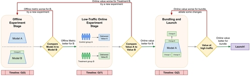
The auction ranking stage has two models: pCTR predicts the click after an impression, pConvs predicts the number of conversions after a click; together with the advertiser's bid they produce the auction score for a second-price auction. The business metric behind launch decisions is Delivered Value (DV):
is the target price per conversion the advertiser is willing to pay (tCPA), is the number of conversions from the -th click. A purchase of a 1,000-dollar mattress is worth more than a hundred visits to a merchant's website, yet an ordinary conversion prediction loss counts both as equal conversions.
The stages take O(X), O(Y) and O(Z) time respectively, with X much smaller than Y and Y much smaller than Z, so every wrong judgment in an earlier stage wastes the more expensive resources of later stages. The authors split measurement error into three kinds: objective misalignment (what an earlier stage measures does not predict the later stage's result), systematic error (bias introduced by the experimental setup), and random error (variance from system noise).
2. Aligning the offline loss with delivered value
2.1 pConvs: Poisson loss weighted by tCPA
pConvs originally did maximum likelihood under a Poisson distribution, with loss , where is the predicted number of conversions for the -th click. The authors changed the prediction target from "conversions after a click" to "delivered value after a click", and the loss becomes the weighted Poisson loss (WPL):
The paper gives a derivation for why the weighting is correct. Let the advertiser's true value be , the bid , and the second price (what the advertiser actually pays) have density $f(s)$; the expected profit of one auction is the integral of "value minus cost" over winning outcomes, . If , the integral comes out as plus a constant, so maximizing profit is equivalent to minimizing ; substituting and back and dropping parameter-independent constants gives WPL. Poisson regression works here not because conversion counts really follow a Poisson distribution, but because the 1/s cost distribution approximately holds.
2.2 pCTR: from "whether clicked" to "how many clicks"
pCTR originally predicted the probability that an impression is clicked at least once, trained with log loss and evaluated with AUCLoss (1 minus AUC). A carousel ad impression often gets several clicks, and each extra click has value, so the team changed the target to the expected number of clicks per impression, raising online DV by 1.2%.
This change is almost invisible offline:
| Offline metric | Change |
|---|---|
| Binary AUCLoss | -0.10% |
| Multi-class AUCLoss | -0.15% |
| LL | +0.08% |
| PL_CTR | -0.21% |
Log loss even got worse; only the Poisson loss computed on click counts, PL_CTR, dropped clearly, matching the direction of the 1.2% online gain.
pCTR also needs to carry value, but using conversion value directly as the weight fails because too few clicks have conversions and the labels are an order of magnitude sparser. The authors instead use expected delivered value as a proxy, with each impression weighted by , giving , where is the number of clicks on the -th impression. The appendix uses the assumption that the runner-up's effective cost-per-thousand-impressions bid follows a $1/r$ distribution to give a derivation of the same form as 2.1.
2.3 Results after switching objectives
This experiment is meant to show two things: WPL as an offline metric better predicts online value, and training on WPL directly raises value.
| Model | PL change | WPL change | Online DV |
|---|---|---|---|
| pConvs trained on WPL | +0.1% | -0.35% | +3% |
| pCTR trained on WPL | +0.03% | -0.04% | +0.5% |
For both models PL got worse, WPL got better, and online DV went up, which shows that what PL measures points in a different direction from the business objective.
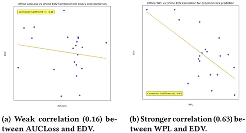
Correlation is measured as follows: over the same set of changes, compute the Pearson correlation between the change in the offline metric and the change in online DV (absolute values are reported below). For pConvs, over about 40 experiments with online data, PL's correlation is 0.1 and WPL's is 0.65 (p<0.01); over 25+ later new experiments it is close to 0.69. For pCTR, over 25 experiments in the "whether clicked" phase, the correlation with EDV is 0.16 for AUCLoss and 0.09 for log loss; over 20 experiments after switching to expected clicks, multi-class AUCLoss reaches 0.33 and 0.63. Computed directly against the noisier DV, the correlation rises from 0.26 to 0.44.
3. Offline stage: systematic and random error
All models are trained continuously online, each example passes through only once, and offline evaluation uses progressive validation: each example is first predicted and its loss recorded, then used for training.
Systematic error has two sources. The first is label maturity bias: conversion labels arrive with delay, the experiment model starts later than the control, and while catching up on historical data it sees more complete conversion labels, so its loss over the same time period looks better only because it has more information; the fix is to compare only over periods where the two models' training data have the same quality. The second is optimizer artifacts: with second-order optimizers and architectures like DLRM that group features for interaction, adding one constant feature can change the grouping and split important features that need to interact into different groups. After fixing these two, the offline difference between two equivalent models stays within 0.02%, where previously significant differences were often measured.
Random error is suppressed by standardizing the measurement method. The table below compares, over 25 pConvs experiments, the offline-online correlation and the AUC-ROC of using the offline result to judge whether the online result is good, when the offline metric is measured over different time windows. is each experiment's launch time.
| Offline measurement window | Correlation | AUC-ROC |
|---|---|---|
| [T−6 months, T−3 months] | 0.650 | 0.760 |
| [T−1 month, T] | 0.577 | 0.690 |
| [T−1 week, T] | 0.01 | 0.489 |
| Same fixed 3 months for all experiments | 0.640 | 0.755 |
| [T, T+online experiment duration] | 0.604 | 0.736 |
Looking only at the last week, the correlation is close to 0 and AUC-ROC is below 0.5, worse than random guessing; a 3-month window beats a 1-month one. WPL weights range from 0.01 dollars to 1,000 dollars and are very noisy; capping the weights at the same upper limit used for DV capping halves the confidence interval without introducing bias.
4. Online stage: the small-traffic control must be as small as the experiment
4.1 Systematic error comes from different traffic sizes
The common practice is to compare the small-traffic experiment model against the large-traffic production model, which is necessarily biased. There are three reasons: a small-traffic model sees little of its own traffic during continuous training and cannot correct its own prediction bias, which is the winner's curse; advertiser budgets are fixed, and under small traffic the budget constraint barely binds, so value is overestimated; under large traffic, feedback control pulls prediction bias back toward the target constraints, and small traffic lacks this correction.
The authors' approach is to set a standard small-traffic size and retrain a copy of the production model at that traffic size, as a shared control for all experiments of that size. When another traffic size is needed, a separate control of that size is trained. After the change, the DV difference between two identical retrained models is close to 0%, where it used to often exceed 1%.
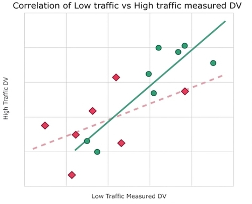
This comparison uses 7 historical experiments (old setup) and 8 new experiments (new setup); the small-to-large traffic correlation rose from 0.53 to 0.93. The sample is small because large-traffic experiments are expensive, but each large-traffic experiment runs long with a lot of traffic, so each single measurement is itself precise. The two groups evaluate the same set of models and are correlated at about 0.75 with each other; the authors use a Williams t-test that accounts for this correlation and get p<0.05.
4.2 Random error: capping and expected values
DV depends on sparse conversions, so its confidence interval is wide. Capping large per-click values shrinks the confidence interval width by 40% with bias under 3%; replacing actual DV with expected DV (pConvs predictions in place of actual conversions) shrinks the width by another 70% with bias of about 5%. Combined, the width shrinks by about 82%, and a 2%-traffic experiment now reaches the precision of a former 30%-traffic experiment, so the same traffic can run more experiments in parallel.
5. Why correlation determines efficiency
The authors assume that offline and online results follow a correlated bivariate normal distribution; multiplying the probability that the offline judgment agrees in direction with the next stage by the probability that the small-traffic judgment agrees with large traffic gives the probability that both judgments are correct:
is the offline-to-small-traffic correlation and the small-to-large traffic correlation. Before the improvements they were 0.1 and 0.53, giving a probability of about 0.36; after, about 0.69 and 0.93, giving about 0.65.
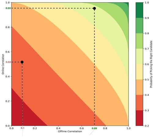
The text gives the improved offline correlation as 0.65 while the figure marks 0.69; by the formula, 0.69 corresponds to a probability of about 0.65 and 0.65 to about 0.64. The paper's efficiency evidence is 100+ experimental changes over 3 years: the number of successful changes included in each bundled pConvs launch, and the number of changes per contributor, both kept rising; the authors estimate overall efficiency roughly doubled, with exact numbers withheld for confidentiality.
6. Limitations
The authors acknowledge that all evidence comes from a single continuously trained online environment, Google Discover ads. The WPL derivation relies on costs following a $1/s$ distribution; the authors note in the appendix that the actual runner-up bid distribution decays faster with a lighter tail, and leave cost distributions closer to reality for future work.
In addition, DV itself is a simplified metric the paper uses to illustrate the problem; real launches look at several interdependent metrics, and the small-to-large traffic correlation is based on only 7 and 8 experiments.
7. Practical implications
- If your model serves an auction ranked by bids, try multiplying the offline evaluation loss by each example's business value and check whether its correlation with online results improves; without changing training, this tells you whether your current offline metric is measuring the wrong thing.
- A small-traffic experiment's control should be the same size and retrained the same way as the experiment arm. Comparing a small-traffic experiment arm against the large-traffic production model mixes winner's curse, budget and feedback-control biases into the measured difference, and an A/A experiment can catch this first.