Contents · 8 sections
1Two kinds of vectors in two clusters2Where the reasoning comes from3Both versions as positives4Walking through it: one query, two positives, one negative5Stage 2: teaching the fast branch what the reasoning branch knows6Results7What this means for people building retrieval8LimitationsSHARE

Reasoning before encoding is more accurate, but the two kinds of vectors drift apart: how AntEmbed lets fast and slow retrieval share one indexGive a multimodal retrieval model an image and ask it which category the image belongs to. The fastest way is to read the image, encode it as a vector, and compare that vector with the ones in the library. The slower way is to let the model first write a piece of reasoning, such as "the classification intent of this image is ... Answer: a perfume product", and then encode that text together with the original image.
The second way is usually more accurate on complex, fine-grained retrieval, but a piece of text has to be generated before every encoding. In a real system you would want to take the fast path most of the time and switch to the slow one for hard queries. The two vectors encoded from the same image, though, can sometimes sit fairly far apart.
This paper, from Soochow University and Ant Group, builds a multimodal embedding model that supports both modes and puts both kinds of vectors in the same space. The kind produced without intermediate content is called a discriminative embedding; the kind produced by reasoning first and then encoding is called a generative embedding. UME-R1 is an existing dual-mode multimodal embedding model: the two modes encode separately, each with its own embedding token. The two kinds of vectors tend to drift apart, and retrieval then needs a separate index for each mode. AntEmbed uses a single embedding token and lets fast and slow queries share one index. On MMEB-v2 (a multimodal embedding benchmark covering image, video and document retrieval), AntEmbed-8B with reasoning queries reaches an overall score of 81.5, the highest among the compared models.
Treating both versions of a candidate as positives, each compared against the negatives on its own, lets fast and slow queries share one index; but the 81.5 needs reasoning generated at query time, and the fast mode without reasoning still trails Qwen3-VL-Embedding at the same size.
Two kinds of vectors in two clusters
A discriminative embedding sends an image, text or a document screenshot straight into the model and reads the hidden state of a dedicated embedding token that produces the vector. A generative embedding first writes out reasoning and a one-line summary, appends them to the raw input, and then reads the hidden state of an embedding token.
The figure below compares how far apart UME-R1 and AntEmbed place the two vectors of the same instance.
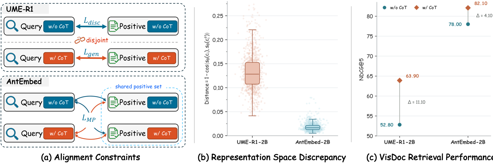
Look at panel (b): for UME-R1-2B the median distance (1 minus cosine similarity) is around 0.13, for AntEmbed-2B only around 0.02. A large distance means the two vectors are offset from each other, and searching a library encoded in one mode with a query in the other mode may suffer.
Panel (c) of the same figure has another set of numbers: on document retrieval, UME-R1-2B scores NDCG@5 of 52.80 without reasoning and 63.90 with it, a gap of 11.10. This shows the information that reasoning adds is useful, and also that the path without reasoning has plenty of room to improve.
Where the reasoning comes from
The reasoning in the training data is written by an external model. The paper uses Qwen3-VL-30B-A3B-Instruct as the reasoner and writes the query side and the candidate side separately.
Query-side reasoning only states the retrieval intent and what evidence is needed, without giving the answer directly. Candidate-side reasoning adds a step: first use the open-source multimodal embedding model Qwen3-VL-Embedding-8B to find the 5 neighbors in the library most similar to this candidate, then give the candidate and those 5 neighbors together to the reasoner and ask it to write "compared with these similar candidates, what makes this one recognizable". The paper calls this confusion-aware, meaning it looks for differences specifically against easily confused candidates. The output may not mention the neighbors; it only describes evidence on the target candidate itself.
Each piece of reasoning has two parts: a reasoning passage plus a short summary, such as "Answer: a perfume product". Both are appended after the raw input.
Both versions as positives
A single token is not enough on its own. Trained with the original objective, the model would still learn two unrelated sets of pairs: original query with original candidate, reasoning query with reasoning candidate. The two sets share one vector space, but nothing requires the original query to be close to the reasoning candidate as well.
AntEmbed puts both the original and the reasoning version of a candidate into the positive set, and both the original query and the reasoning query are compared against that set. One training sample then has four pairs to pull together: original query with original candidate, original query with reasoning candidate, reasoning query with original candidate, and reasoning query with reasoning candidate.
Once there are two positives, how the loss is written matters. The simplest form adds the scores of the two positives and only asks "the positive group" as a whole to beat the negatives. The paper does not use this form; it switches to pairwise comparison, where each positive is compared against each negative separately. Below we compute where the two forms differ.
Walking through it: one query, two positives, one negative
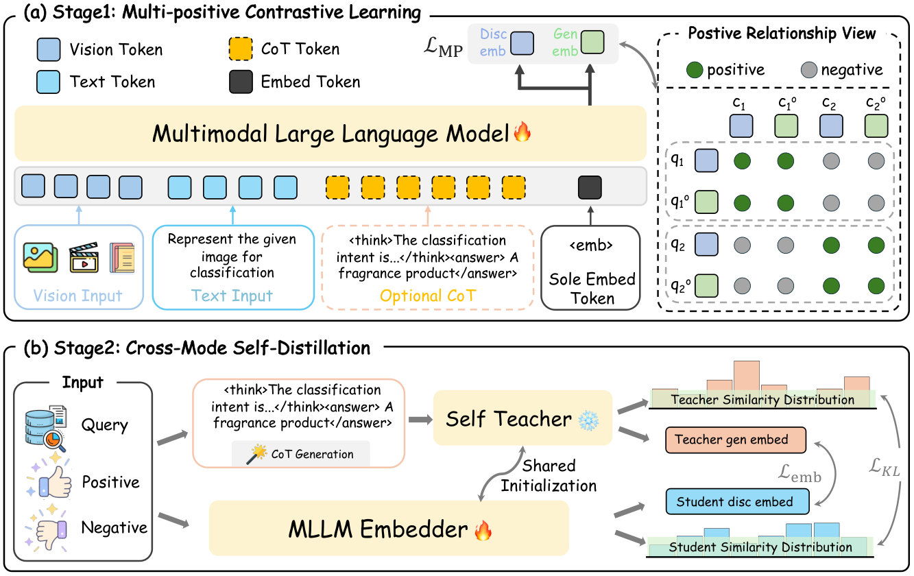
The upper left of this overview figure is the encoding process: an image to be classified, plus the instruction "Represent the given image for classification", with optional reasoning that ends with "Answer: a perfume product", all passed to an embedding token. The small table on the right separately shows the training correspondence: both versions of each query treat both versions of the same candidate as positives. The figure does not label a positive or a negative for this classification example.
The calculation below is a separate, illustrative example of the two loss forms. The temperature 0.02 is the paper's setting; the three similarities are illustrative, not scores measured on this classification figure. Suppose we have one query, two versions of the same candidate as positives, and one negative. The query first takes the path without reasoning and sees only the raw input.
Step 1, the starting point. The original query has similarity 0.8 with the original candidate, only 0.2 with the reasoning candidate, and 0.5 with a negative. In other words, the original query is farther from the reasoning version of its own candidate than from the negative.
Step 2, the loss with "positive scores added". Each score is divided by the temperature first: the positives become 0.8 ÷ 0.02 = 40 and 0.2 ÷ 0.02 = 10, the negative becomes 0.5 ÷ 0.02 = 25. The numerator is e^40 + e^10, almost entirely decided by e^40; the negative's e^25 is smaller than e^40 by a factor of e^15. The loss is about e^-15, close to 0, so the model treats this sample as already learned and leaves the 0.2 alone.
Step 3, the paper's pairwise form. Each "negative minus positive" difference is also divided by the temperature: for the original candidate it is (0.5 − 0.8) ÷ 0.02 = −15, for the reasoning candidate (0.5 − 0.2) ÷ 0.02 = 15. The loss is log(1 + e^-15 + e^15), about 15, which means the same sample, under a different form, goes from "already learned" to a sample with a large loss.
Step 4, where the gradient pushes. Almost all of that 15 comes from the reasoning-candidate term, so the gradient mainly does two things: push up the similarity between the original query and the reasoning candidate, and push down its similarity to the negative. The original-candidate term already wins by 0.3 and contributes almost nothing.
Step 5, the same calculation for the reasoning query. The reasoning query must also beat the negative separately and stay close to both positives. All four pairs are held in place one by one, so the two vectors of the same instance are pulled together. In panel (b) of the earlier comparison figure, the two vectors of AntEmbed-2B are only about 0.02 apart; that is the outcome.
The paper compares the effect of this step in Table 3, on image tasks with the 2B model:
| Training method | Query without reasoning | Query with reasoning |
|---|---|---|
| Original data only | 68.7 | — |
| Reasoning data only | — | 73.6 |
| Both kinds of data mixed | 68.8 | 67.0 |
| One LoRA per kind, then merged | 69.0 | 73.8 |
| Two positives compared one by one | 73.3 | 79.5 |
(Numbers from the paper's Table 3, average over MMEB-v2 image tasks.)
This shows that simply mixing the two kinds of data, or merging the parameters of two models, only matches training each one alone; with mixed training, reasoning queries even drop to 67.0. Among these methods, the one that makes the two versions positives for each other beats separate training by 4 to 6 points in both modes.
Stage 2: teaching the fast branch what the reasoning branch knows
After stage 1, the two kinds of vectors share a space, but reasoning queries are still more accurate. Stage 2, shown in the bottom half of the overview figure, aims to let queries without reasoning pick up part of the information that reasoning brings.
The method is self-distillation. Teacher and student both start from the stage-1 model: the teacher reads the reasoning query, the student reads the original query, and only the student is updated. The distillation has two layers. The first looks at candidate ranking: the teacher computes a similarity distribution over a batch of reasoning candidates, the student computes one over the same batch, and a KL divergence pulls the student's distribution toward the teacher's, with weight 1.0. The second looks at the vector itself: it pulls the student's query vector directly toward the teacher's reasoning-query vector, with weight 0.5.
With the first layer alone, the student learns "which candidate is more similar than which", while the vector itself can stay far from the teacher's; the second layer fills that in. In the paper's Table 4 (all overall scores for queries without reasoning), stage 1 scores 69.1, adding only the first layer gives 69.4, adding only the second gives 69.5, and using both with weights 1.0 and 0.5 gives 70.2. This says the two layers complement each other, but stage 2 trains only on a subset of image and document data, and the gain is about 1.1 points.
Results
The main experiment is on MMEB-v2, with 78 datasets across image, video and document. All candidates go into one library, encoded in their reasoning version; queries come in two modes: without reasoning (base) and reasoning first (CoT).
| Model | Image | Video | Document | Overall |
|---|---|---|---|---|
| Qwen3-VL-Embedding-8B | 80.1 | 67.1 | 82.4 | 77.8 |
| DME-9B | 79.8 | 70.8 | 82.0 | 78.4 |
| AntEmbed-8B, no reasoning | 76.4 | 57.6 | 79.9 | 73.1 |
| AntEmbed-8B, reasoning first | 83.9 | 74.8 | 82.7 | 81.5 |
(Numbers from the paper's Table 1; baseline scores come from the official leaderboard.)
The reasoning mode does lead: its overall score is 3.1 above DME-9B and 3.7 above Qwen3-VL-Embedding-8B, and it is highest in all three categories. The largest gain is on video, where the 2B model rises by 12.8 points from no reasoning to reasoning. The fast mode without reasoning scores 73.1 at 8B, 4.7 points below Qwen3-VL-Embedding of the same size; at 2B it scores 70.2, second among discriminative models only to Qwen3-VL-Embedding-2B at 73.2, but already above models that need reasoning, such as TTEt-2B (68.6) and Embed-RL-4B (68.1).
The strength of the reasoner directly affects the result. When different reasoners write the query reasoning at evaluation time, the 2B model's average on image tasks goes from 73.3 without reasoning, to 78.1 with a fine-tuned Qwen3-VL-8B, to 79.3 with Qwen3-VL-30B-A3B and 80.2 with Gemini-3.1-Pro. Even a smaller reasoner gets most of the gain.
On the broader MMEB-v3, AntEmbed-8B's overall score is 55.6, also the highest among the compared models, and it ranks first in the text and agent categories. AntEmbed does not support audio, and the 11 audio tasks count as 0 in the overall score.
What this means for people building retrieval
If you want a fast tier and a slow tier in the same retrieval system, you can build a single candidate library and let both kinds of query search it.
The key is the training objective: treat the different versions of the same candidate all as positives, and compare each one against the negatives, instead of only looking at the probability of the positives as a whole. The 0.2 example above shows that adding the positive scores lets the model ignore the version that is far away.
In deployment, you can default to the fast query without reasoning and send only hard queries to the reasoning mode. A smaller reasoner still gets most of the benefit, as the 78.1 from the fine-tuned Qwen3-VL-8B shows.
Limitations
Every query in reasoning mode has to wait for the reasoner to finish writing a passage. The paper's tables only compare retrieval quality; latency and cost are outside the comparison. The candidate library is encoded in the reasoning version, so every candidate in it must first go through the reasoner once, which is an extra offline cost.
The fast mode without reasoning still trails Qwen3-VL-Embedding at the same size. Stage-2 distillation adds only about 1.1 points, and it is trained only on a subset of image and document data.
In the MMEB-v3 overall score, audio tasks count as 0, and the baseline scores of the other new tasks are taken directly from the original MMEB-v3 paper rather than re-run in the same environment.
How did this read for you?
Hoot made a note. Thanks for the feedback.

One tap, no sign-in; tap again to undo. Only anonymous counts are kept, never who you are.
Related papersMore from Paper Daily
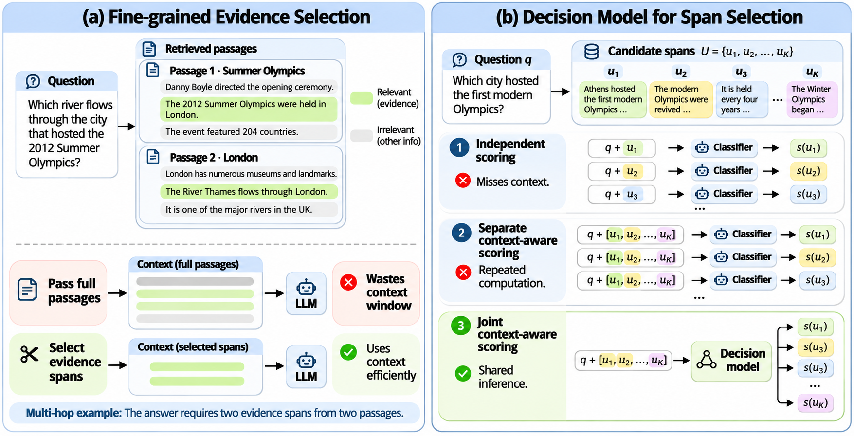 Retrieval · 2026-11-16CURATOR: Scalable Fine-grained Evidence Selection for Retrieval-Augmented Generation using Decision ModelsRAG usually stuffs whole retrieved passages into the LLM, though often only a few sentences in them can answer the question. Picking those sentences is not easy: a sentence can look irrelevant on its own, and whether to keep it may depend on other retrieved text. Judging each sentence with the full context is too expensive. Decision models can score many candidate sentences in one pass, with each…
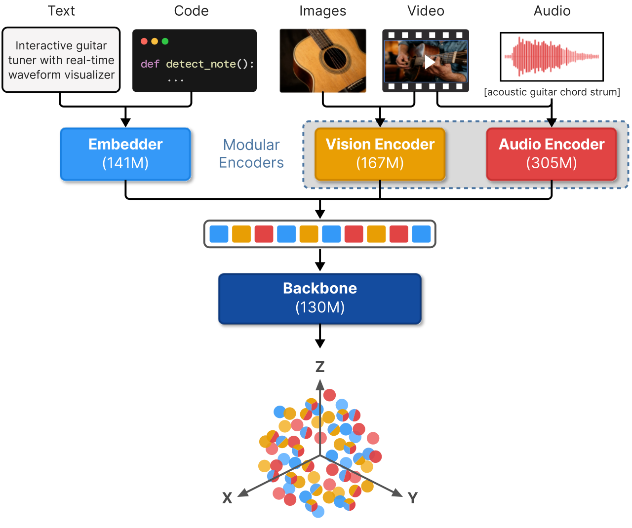 Retrieval · 2026-10-29EmbeddingGemma 2: Unified and Efficient Multimodal RepresentationsTo search text, images, video and audio with one embedding model, the usual route is to transcribe audio and caption images first, then hand everything to a text model. That costs extra compute and throws away tone of voice and visual detail. Google's EmbeddingGemma 2 is a 744M-parameter model that maps these inputs directly into one vector space, and each modality encoder can be loaded only when…
 Retrieval · 2026-11-02Retrieving from Your Own Mistakes: On-Policy Training of Embedding Models for Multi-Hop Retrieval-Augmented GenerationChain embedding retrievers for multi-hop retrieval see different histories in training and in use, and this paper fixes that without adding any LLM call. At each step such a retriever joins the question with the passages found so far to look for the next one; in training its history holds only correct passages, but in use it often holds wrong passages it found itself. On four-hop MuSiQue question…
Discussion
Add experiment details, reproduction notes or a different take. Requires a GitHub sign-in.
Loading the discussion…