Contents · 9 sections
1What problem is it solving?2The core idea: group by similarity, not by position3How does a query choose candidates?4How is the index built during computation?5Why learn the representatives?6Results7Limitations as I see them8How a long-context serving team could try it9VerdictSHARE

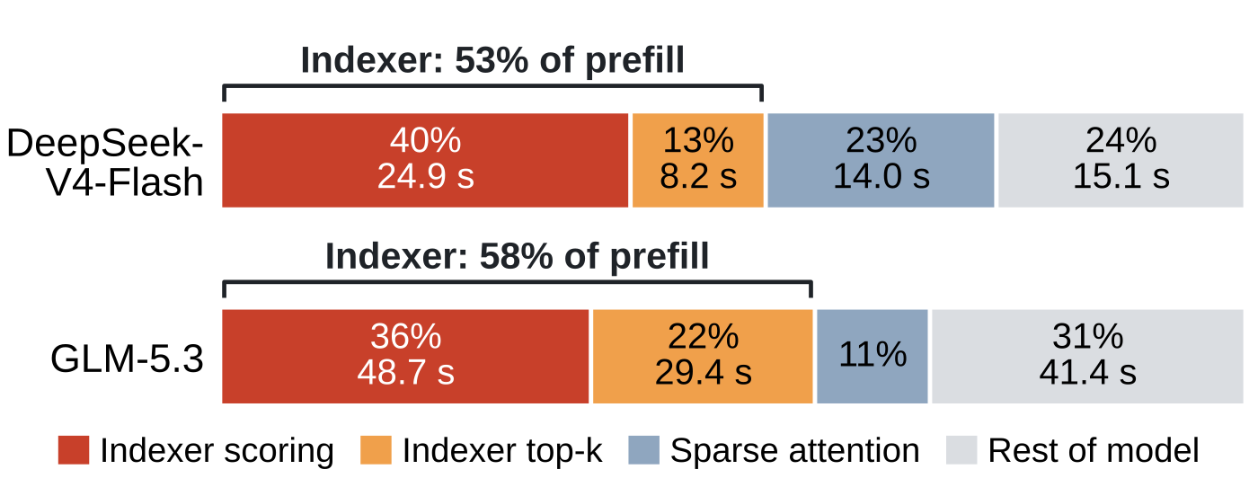
In learned sparse attention, as used by DeepSeek-V4 and GLM-5.3, each query attends to only k keys, but the small scoring network that picks those k keys still scores every key in the prefix. At one million tokens, that step takes 53% to 58% of prefill time. AttentionIndex sharply cuts this cost. During prefill it groups keys by similarity; a query first scores one representative per group, and only the members of the most promising groups go to the original scoring network for the final pick. At that length, its prefill throughput is 1.3 to 1.8 times that of scoring every key; against HiSA, a block-based method at similar speed, it recovers 17.0 (GLM-5.3) and 10.0 (DeepSeek-V4-Flash) percentage points more of the keys that should have been selected.
What problem is it solving?
First, how this kind of sparse attention works. DeepSeek Sparse Attention (DSA) adds a lightweight scoring network to the model, which the paper calls the indexer. For every query token, in prefill and decoding alike, the indexer scores every earlier key, and the main attention looks only at the k highest-scoring ones (2,048 on GLM-5.3). The cost of the main attention no longer grows with context, but the indexer's own scoring does. Section 3.1 measures a one-million-token prefill: indexer scoring plus top-k selection take 53% on DeepSeek-V4-Flash and 58% on GLM-5.3, more than the rest of the model combined, and 2.4 and 5.2 times the time spent in sparse attention itself.
The natural way to save this step is to pick in two stages: first select a batch of candidate keys coarsely, then let the indexer pick precisely among the candidates only. The maximum number of candidates is what the paper calls the candidate budget. The existing method HiSA cuts the keys into contiguous blocks by position, uses each block's average as its representative, and keeps the blocks whose representatives score highest. The trouble is that keys next to each other need not be similar. A block may hold only two or three important keys; averaged together they score low, the whole block is dropped, and the precise stage can never get them back. The longer the context, the more blocks compete and the worse this gets. In Table 1 of the paper, with 8K candidates on GLM-5.3 and LongBench-v2, the share HiSA recovers falls from 83.9% at 16K context to 41.8% at 256K.
This "share recovered" is an evaluation metric, which the paper calls recall: offline, the indexer scores all keys, its top k become the reference answer, and recall is how much of the coarse-plus-precise result falls inside that reference. At inference time the system never knows the reference answer; it is only used for comparison at evaluation time.
The core idea: group by similarity, not by position
AttentionIndex starts from one observation: the precise stage already scores every candidate exactly, so all error comes from keys missed by the coarse stage. If groups are formed by content, the important keys concentrate in a few groups, and the same candidate budget holds more of the keys that should be selected.
This is exactly what an inverted-file (IVF) index does in vector search. In this paper, the items being grouped are the indexer's keys, each group is a set of similar keys (the paper calls it a cluster), and each group takes part in the coarse pass through one representative vector.
Bringing IVF into attention raises three difficulties, and the paper answers each:
| Difficulty | Why it is hard | What AttentionIndex does |
|---|---|---|
| The index must be built during computation | Every stretch of prefill adds new keys, and rebuilding the index each time may cost more than the scoring it saves | New keys first go into an "ungrouped area" and are grouped once a batch is full; every so often the whole prefix is regrouped, reusing the previous result |
| No peeking at later text | Each query may only see the keys before it, and representatives must not mix in later keys | Each grouping creates a new index version, and a query uses it only if its prefix already contains all of that version's keys |
| The average is a poor label | The indexer score is not a plain inner product, so the score of a group's average does not stand for its members' scores | A small network trained offline adds a correction to each group's average, and the corrected representative is used for the coarse stage |
How does a query choose candidates?
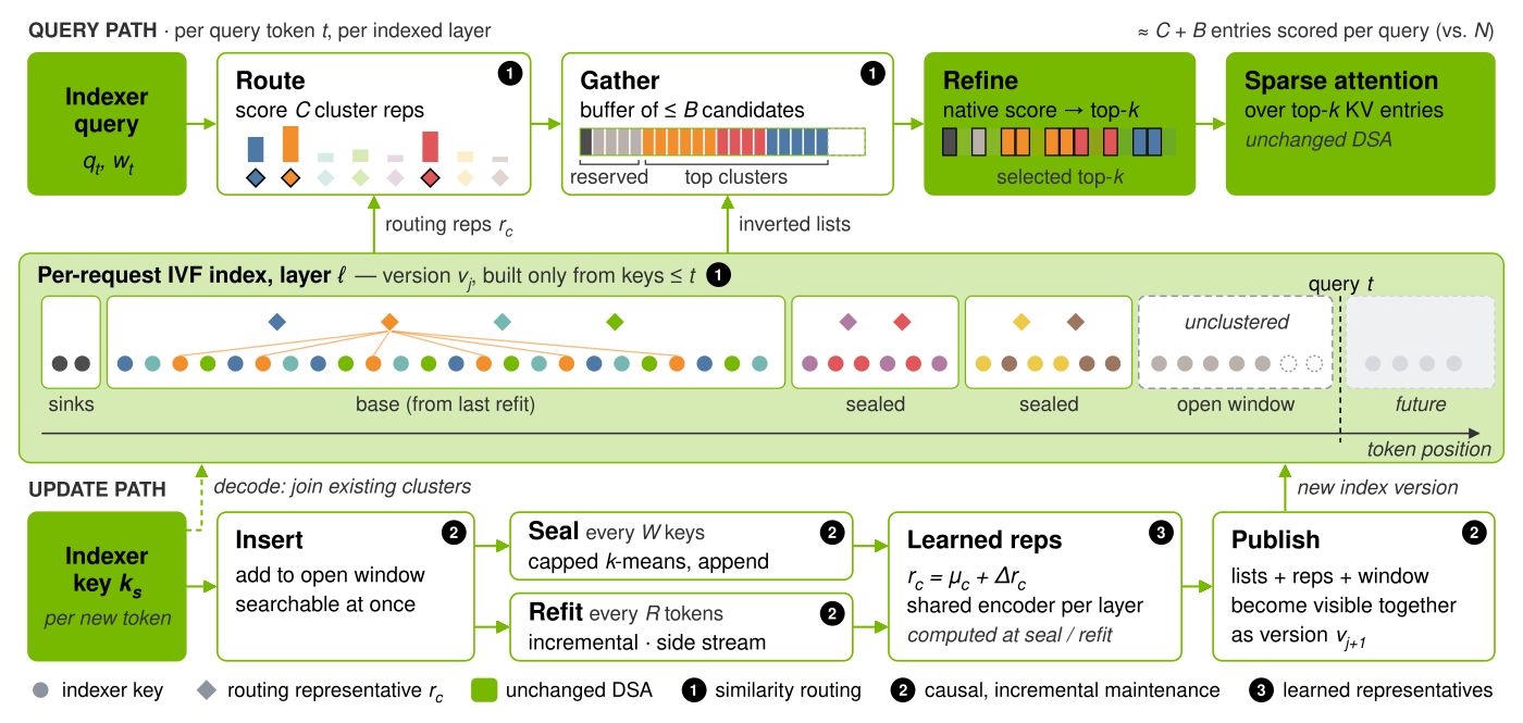
Each query first uses the indexer's original scoring formula on every cluster representative and ranks the clusters. Then it fills the candidates: the first few keys and the not-yet-grouped new keys take fixed slots, and the remaining slots take all members of each cluster in rank order, cutting off the last cluster if it does not fit. The indexer then scores these candidates one by one and passes the top k to the original sparse attention.
So each query scores roughly "number of clusters plus candidate budget" entries instead of N, the prefix length. On GLM-5.3 a cluster holds about 128 keys, so the number of clusters is about 1/128 of the prefix length. The coarse stage still grows with the prefix, but with a much smaller constant. The sparse attention computation itself is unchanged.
How is the index built during computation?
Prefill moves forward chunk by chunk, and each step adds keys to the prefix. AttentionIndex splits maintenance into three levels:
- Insert. A new key enters the ungrouped area as soon as it is produced. Later queries put the whole ungrouped area into their candidates, so new keys can be selected immediately.
- Seal. Each time the ungrouped area collects W keys, they are grouped and the result is appended; existing groups are not touched. On GLM-5.3, W is 1,024, split into 8 groups of about 128. Before the first seal, queries still score every key.
- Refit. Sealing groups only within one batch, so similar keys from different batches end up in different groups. Every R tokens (16,384 on GLM-5.3), the whole prefix is regrouped, with more groups as the prefix grows.
A refit does not start from scratch. Consecutive refits share almost all their keys, and a key never changes once generated. So a refit starts from the previous group centers plus a few new centers drawn from recent keys. Each key also keeps an upper bound on its distance to its own center and lower bounds on its distances to other centers; only new keys and keys whose bounds no longer settle their membership are compared with every center. Each refit does a single assign-and-update pass rather than running to convergence. Refits run on a separate CUDA stream, in parallel with the normal forward pass.
One more detail prevents peeking at later text. Every seal or refit creates a new index version whose members, representatives and ungrouped-area information take effect together. A query uses a version only if its prefix already contains every key in it. Within one prefill chunk, earlier queries keep the old version and cover newer keys through their own ungrouped area.
Why learn the representatives?
Ordinary IVF uses the group average as the representative. That works for inner-product search: a query's inner product with the average equals the average of its inner products with the members. The indexer score, however, takes an inner product per head, passes it through ReLU, and adds the heads up with weights, so the average's score is no longer the average of the members' scores. A group may contain several keys that should be selected while its average still scores low. Hoot says

Ordinary IVF: average the members, then score
- Members (illustrative)
- −2, 2
- Representative = average
- 0
- Representative score at query = 1
- ReLU(1×0) = 0
The coarse pass sees 0, so the group is skipped.
Scoring every key: score each member first
- Member scores
- ReLU(−2) = 0, ReLU(2) = 2
- Average score
- 1
- Should it be picked?
- the key scoring 2 should be
The group does hold a good key; the average hid it.
This paper: learn a correction added to the average
- Offline
- train the small network so representatives rank groups like "reference keys in group ÷ group size"
- When it runs at inference
- once, only when a seal or refit creates new groups
- What each query does
- scores the representatives as usual, without re-summarizing members
The correction starts at 0, so it begins as ordinary IVF.
Illustrative numbers: one head with weight 1, and the query and keys reduced to single numbers. The real indexer has several heads and longer vectors, but the cancellation works the same way. Source: paper method section: indexer score = per-head inner products through ReLU, then a weighted sum; ordinary IVF uses the group average. Numbers are illustrative.
The paper keeps grouping by distance and corrects only the representatives used for the coarse stage. One small network shared by a layer reads a few summaries of a group's members. These are the average of the member keys, the log of the group size, and features made by passing each member key through a small learned transform and then taking the average and the maximum of the results. Training and inference use the same network and the same summaries. It outputs a correction that is added to the average. The correction is bounded and starts at 0, so at the start it equals ordinary IVF. The network is trained offline: run a batch of queries through the frozen model, take the top k from scoring every key as the reference answer, and make the representatives rank groups as closely as possible to "reference keys in the group divided by group size". At inference time it runs only when a seal or refit creates new groups, and queries score the representatives as usual.
Results
The experiments use SGLang on eight B200 GPUs with GLM-5.3 and DeepSeek-V4-Flash; the baselines are scoring every key (Full DSA) and HiSA. The candidate budget counts tokens on GLM and compressed entries on DeepSeek-V4-Flash (each entry covers 4 original tokens).
First, recall. On all three datasets and at every budget, AttentionIndex beats HiSA. LongBench-v2 at a 24K budget, for example:
| Model | HiSA | AttentionIndex |
|---|---|---|
| GLM-5.3 | 67.16% | 89.70% |
| DeepSeek-V4-Flash | 75.88% | 90.66% |
It wins even with fewer candidates: on GLM-5.3, its results with 24K candidates beat HiSA's with 64K on all three datasets, using 62.5% fewer candidate slots. This is consistent with the idea that grouping by content concentrates the keys that should be selected into fewer groups.
Next, speed. When every key is scored, throughput drops by more than half as context grows from 256K to one million tokens. At one million tokens, AttentionIndex's prefill throughput is 1.6 to 1.8 times that of scoring every key on GLM-5.3 and 1.3 to 1.6 times on DeepSeek-V4-Flash. At shorter contexts the index does not yet pay off: it is at least as fast as scoring every key at all budgets only from 384K on GLM-5.3 and 512K on DeepSeek-V4-Flash. At the same budget it is faster than HiSA on GLM-5.3 up to 512K to 768K tokens, but slower beyond that and on DeepSeek-V4-Flash, because it maintains the index and gathers candidates from scattered positions. So the fair comparison aligns speed first and then compares recall (Table 2 of the paper, throughput within 5%):
| One million tokens | HiSA budget | HiSA recall | AttentionIndex budget | AttentionIndex recall |
|---|---|---|---|---|
| GLM-5.3 | 24K | 69.6% | 16K | 86.6% |
| DeepSeek-V4-Flash | 24K | 76.5% | 16K | 86.5% |
At similar speed it uses a third fewer candidates and still recovers 17.0 and 10.0 percentage points more.
Last, task accuracy (Table 4). At the same 24K budget, AttentionIndex beats HiSA on all three benchmarks for both models. The largest gap is on RULER: from 62.6% to 77.5% on GLM-5.3, where scoring every key gives 81.8%; from 67.27% to 76.14% on DeepSeek-V4-Flash, where scoring every key gives 77.83%. On LongBench-v2 the difference is small, because HiSA was only 2.8 and 0.80 points behind scoring every key in the first place. The paper's explanation is that this benchmark tests reasoning over long text, so model capability may become the bottleneck no matter how well the keys are chosen. At matched speed (AttentionIndex 16K against HiSA 24K), it wins four of the six comparisons; on LongBench-v2 it is 0.6 and 1.39 points lower.
Two ablations. Turning off refits and relying only on seals drops GLM-5.3's recall at a 24K budget from 88.3% to 78.8%, with all 13 inputs getting worse, so regrouping across batches matters a lot. Learned representatives raise recall by 0.55 to 5.01 points on four GLM-5.3 layers but only about 0.2 points on two DeepSeek-V4-Flash layers, and change time to first token by at most 1.6%.
Limitations as I see them
First, decoding does worse than HiSA. When a long prefill joins a batch that is generating, AttentionIndex gives a 1.40 to 1.45 times speedup in time per output token over scoring every key, versus 1.54 to 1.65 times for HiSA. The paper leaves decoding cost to future work.
Second, maintenance grows with the prefix. Each refit revisits every key in the prefix, and on GLM-5.3 beyond 512K to 768K tokens it is slower than HiSA at the same budget. At about one million tokens and a 24K budget, index construction, refits, candidate packing and cross-GPU exchange take 15% of GPU work on GLM-5.3, more than all scoring and top-k combined (including coarse-stage scoring, 11%). These figures sum GPU work on parallel streams and are not extra request latency, but they show that a good part of the saved scoring is spent on maintenance.
Third, the learned representatives give uneven gains. Of the five DeepSeek-V4-Flash layers evaluated, only two enable learned representatives, each gaining about 0.2 points; the other three keep the plain average. The paper suspects this relates to compressed entries mixing neighboring tokens, but does not test it separately.
How a long-context serving team could try it
- Confirm the bottleneck first. If you serve long contexts of hundreds of thousands of tokens with models like DeepSeek-V4 or GLM-5, profile one prefill and check the share taken by indexer scoring plus top-k. Below 256K context, the paper's results say the index does not yet pay off.
- Start with sealing only. Group every 1,024 new keys into 8 groups, keep only the top-ranked groups in the coarse stage, and compute recall against scoring every key with offline replay.
- Then add refits. Regroup the whole prefix every 16K tokens and check whether recall rises by about 9 points over seal-only (Table 5 of the paper: 78.8% to 88.3% on GLM-5.3 at a 24K budget).
- Consider learned representatives last. They need offline training and their gain varies by layer, so try them only on the few layers with the lowest recall.
Verdict
The key lesson: once sparse attention holds down the cost of attention itself, choosing the keys becomes the new bottleneck; and because all the error in choosing comes from the coarse stage, grouping by content uses a limited candidate budget better than cutting blocks by position.
| Dimension | Assessment |
|---|---|
| Importance | High. At one million tokens, choosing keys takes over half of prefill, which long-context agent and code workloads will hit |
| Novelty | Medium-high. IVF and bound-based k-means speedups already exist; the new part is putting the index inside a single request's forward pass without peeking at later text |
| Evidence | Fairly strong. Two real models, three benchmarks, speed-aligned comparisons and two ablations, but decoding is tested only at 2 to 4 concurrent requests |
| Engineering cost | Fairly high. It changes candidate selection in the serving framework and syncs index state across GPUs, and learned representatives need offline training |
| Worth trying | Worth watching. Services dominated by million-token prefills gain the most; decoding-heavy services should wait for follow-up work |
How did this read for you?
Hoot made a note. Thanks for the feedback.

One tap, no sign-in; tap again to undo. Only anonymous counts are kept, never who you are.
Discussion
Add experiment details, reproduction notes or a different take. Requires a GitHub sign-in.
Loading the discussion…