Contents · 9 sections
1What problem is it solving?2The pipeline: find impressions that look like the candidates', then count them more3Where do the weights come from?4Why train only one shared model?5When should you not trust the offline result?6Experiments: clear gains in simulation, near-tied candidates in production7Limitations as I see them8How a recommendation or search team could try it9VerdictSHARE

Before an ad system launches a new ranking model, it must pick the best candidate offline from logs. In multi-stage delivery, impressions pass through auctions, filters and caching, and their selection probabilities are never logged, so IPS cannot be used. The usual substitute scores new policies with a click-predicting reward model, but new policies push impressions toward ads that are rare in the logs, where that model is least accurate. The authors replay the candidates on past requests and train a classifier to tell whether an impression comes from the logs or from a given candidate. For each logged impression, the classifier gives the ratio of its probability under each candidate to its probability under the logs. The average of these ratios over all candidates becomes its weight when training one shared reward model, so impressions that look like what the candidates would show count more. Five candidates in a production CTR ranking system all ran in A/B tests. Picking a winner on each of 50 random log subsamples, the rate of picking the truly best one rises from 0.36 without weighting to 0.40.
People who run offline evaluation for ads or recommendation should read this, and the reason is not the four-point gain. The paper puts a number on a problem many teams sense but never measure: offline evaluation is least trustworthy exactly where the new model disagrees most with the old one. It offers a computable diagnostic, the share of a candidate's impressions that the logs have barely seen, and uses it to decide whether a batch of candidates can be judged offline or should go straight to A/B. The production evidence is weak: the best and second-best candidates are nearly indistinguishable in the offline estimates, and the authors admit offline evaluation cannot separate them.
What problem is it solving?
Without selection probabilities, offline model picking usually relies on DM, which in multi-stage delivery is often the only option.
The catch is that the reward model learned from the old model's impressions. Take an illustrative example: for one kind of request, 95% of logged impressions are game ads and 5% are education ads. Candidate A behaves much like the old model, while candidate B swaps half of its impressions to education ads.
| Illustrative | Share in logs | Candidate A | Candidate B |
|---|---|---|---|
| Game ads | 95% | 93% | 50% |
| Education ads | 5% | 7% | 50% |
The reward model has seen many clicks on game ads and predicts them well. Education ads are rare, so its predictions there may be too high or too low. Half of B's estimated value therefore rests on the region where the reward model is least sure. Worse, this error is not the same size for A and B, so their order can flip. The authors call this policy-induced distribution shift.
The pipeline: find impressions that look like the candidates', then count them more
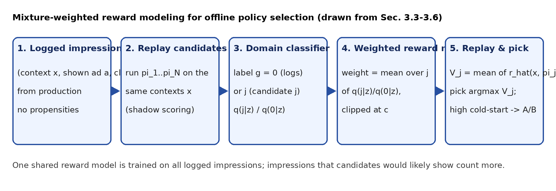
There are five steps. Take the logged impressions. Replay each candidate on the same historical requests to re-choose ads (shadow scoring in the production experiment, offline re-running of the candidate's scoring function in simulation; the ad a candidate picks is taken as its impression, and the paper assumes candidates can be replayed this way). Train a classifier to tell whether an impression came from the logs or from which candidate. Turn the classifier's outputs into sample weights for the logged impressions and train a reward model. Finally, on a separate held-out evaluation split, the reward model predicts the click rate of the ad each candidate picks on each historical request; the average is that candidate's estimated value, and the highest one is picked. The key division of labor: the classifier only answers whose impression this looks like, and the reward model only predicts clicks. Now the parts one by one.
Where do the weights come from?
The obvious idea is a ratio for each logged impression: its probability under a candidate divided by its probability under the logs. Impressions that candidates show often and the logs show rarely get a large ratio and count more in training, so the reward model learns harder in the region candidates care about. But neither probability can be computed, which is exactly why IPS fails.
The authors sidestep this with a multiclass classifier. Real logged impressions are class 0, and impressions that candidate j produces on the same requests are class j. The classifier reads an impression (user features plus ad features) and outputs a probability for each class. With equal numbers of samples per class, the probability of candidate j divided by the probability of the logs equals that ratio we could not compute.
A worked example (illustrative), with two candidates. For one logged impression the classifier outputs 0.25 for the logs, 0.5 for candidate 1 and 0.25 for candidate 2. The two ratios are 2 and 1, and their average gives a weight of 1.5. For another impression it outputs 0.5, 0.25 and 0.25, so both ratios are 0.5 and the weight is 0.5. The first impression looks more like what candidates would show and counts three times as much in training.
When the classifier is sure an impression does not look like the logs, the denominator is tiny and the weight explodes. So weights are clipped at a cap c, 100 in simulation and 20 in production. The authors compared c values of 1, 5, 10, 20 and 100 in simulation. Between 10 and 100 the value error is nearly the same. With c=1, every weight above 1 is pushed down to 1, so only down-weighting remains and no up-weighting; it behaves like the unweighted model when overlap is poor and has the lowest value error only when overlap is high.
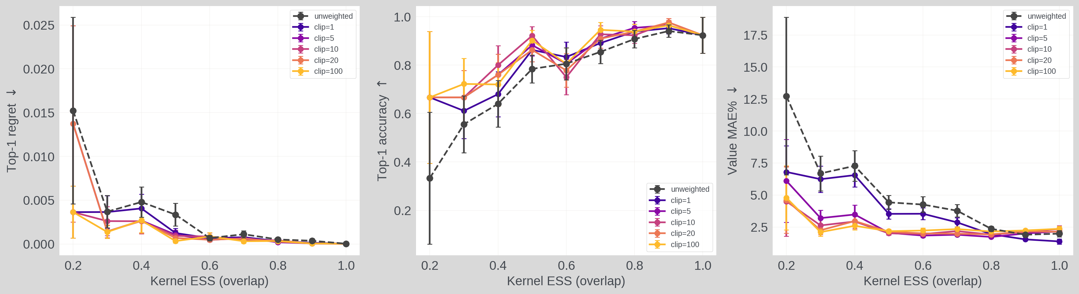
The horizontal axis of this figure is the effective sample size as a share of the sample count. Near 1, candidate and logged impressions look alike; near 0, a few samples carry huge weights and the two are far apart.
Why train only one shared model?
A more natural option is to weight separately for each candidate and train one reward model per candidate, and the paper uses this as a baseline. The authors aim for something else: one reward model that is as accurate as possible across the impressions all candidates would show. So they average the ratios over candidates, train a single model, and let every candidate be scored by it.
The experiments back this choice. In simulation, the shared weighted model beats per-candidate weighting on all nine comparisons. In production, the per-candidate version picks the right winner only 0.24 of the time, as low as IPS. So the gain cannot be explained by training more models.
When should you not trust the offline result?
The theory section splits each candidate's value error into three parts: reward-model error in the region the logs cover; the part of the candidate's impressions the logs have barely seen; and sampling error from a finite evaluation set.
The authors call the second part the cold-start mass: among the impressions a candidate would show, the share whose probability of belonging to the logs is below a threshold (0.1 in the experiments), meaning the logs support them only weakly. The cold-start term in the bound does not vanish as logs grow. If the reward model's fitting, optimization and weight-estimation errors also go to zero, the other terms vanish, and the loss from a wrong pick (the true click-rate gap between the truly best candidate and the chosen one) is then bounded by twice the largest cold-start mass across candidates. That gives a rule: for an acceptable loss, trust the offline pick if the largest cold-start mass in the candidate set is small enough, and otherwise send the whole set to A/B.
This rule is an asymptotic result that holds only with enough data. Estimating cold-start mass with the classifier also requires calibrated classifier probabilities.
Experiments: clear gains in simulation, near-tied candidates in production
The simulation uses the authors' open-source ad simulator: 10,000 users and 1,000 ads, with 10 random candidate ads per request, and the policy picks the highest-scoring one. True click rates come from a known function, so every candidate's true value can be computed. Each trial's 70,000 impressions are split four ways, for training the classifier, training the reward model, calibration and evaluation, over 50 random seeds. There are three metrics: Top-1 accuracy, regret, and the mean percentage error of the value estimates.
The table below groups results into three levels of overlap between candidates and logs, with Top-1 accuracy and value error. The DR rows use the same classifier weights.
| Method | Low overlap acc. | Low overlap error % | Mid overlap acc. | Mid overlap error % | High overlap acc. | High overlap error % |
|---|---|---|---|---|---|---|
| IPS (classifier-estimated ratios) | 0.60 | 7.64 | 0.65 | 5.49 | 0.71 | 4.15 |
| Unweighted DM | 0.67 | 7.20 | 0.87 | 2.58 | 0.96 | 1.59 |
| Weighted DM | 0.81 | 2.65 | 0.91 | 1.94 | 0.98 | 1.86 |
| Per-candidate weighted DM | 0.75 | 3.61 | 0.83 | 2.80 | 0.90 | 2.32 |
| Unweighted DR | 0.82 | 2.64 | 0.93 | 0.70 | 1.00 | 0.30 |
| Weighted DR | 0.90 | 1.71 | 0.95 | 0.43 | 0.99 | 0.21 |
At low overlap, cold-start mass is about 43%, and weighting lifts DM's accuracy from 0.67 to 0.81 while cutting error from 7.20% to 2.65%. At high overlap, cold-start mass is about 12%, and weighted DM's error is slightly higher than unweighted. This shows that weighting pays off when the new model changes a lot; when changes are small, the extra variance from weighting costs a little.
The production experiment comes from a large-scale CTR ranking system with one old model and five candidates, all six of which ran in real A/B tests, so true click rates are known. A random pick would be right 0.20 of the time.
| Method | Top-1 accuracy | Value error % |
|---|---|---|
| IPS | 0.24 | 4.14 |
| Unweighted DM | 0.36 | 14.10 |
| Weighted DM | 0.40 | 11.56 |
| Per-candidate weighted DM | 0.24 | 12.43 |
| Unweighted DR | 0.38 | 1.90 |
| Weighted DR | 0.44 | 2.04 |
Weighted DR picks right most often, but its value error is slightly higher than unweighted DR, so neither clearly wins. IPS has low value error yet picks barely better than chance. Estimating values accurately and picking the right winner are different things: when candidates are close, a few percent of value error is enough to flip the order.
Limitations as I see them
First, the production evidence cannot separate the winner. Weighted DM's top two candidates are nearly equal, and they swap order in 24 of 50 subsamples. This means the rise from 0.36 to 0.40 rests on a nearly tied set, and the authors themselves conclude this set should go to A/B.
Second, weight quality depends entirely on whether the classifier can see policy differences. In the appendix, ad features shown to the classifier are masked step by step. With two thirds masked, weighted DM's accuracy falls from 0.90 to 0.83 and IPS from 0.62 to 0.33. The classifier's log loss and its accuracy at naming the right candidate get worse too, which signals that it is losing the ability to tell policies apart. The subtler trap is the effective sample size share: with all ad features masked it rises from 0.59 to 1.00, because the weights flatten when the classifier cannot see ad features, not because overlap improves. So a high share means good overlap only when the classifier can tell the policies apart.
Third, the routing rule has not been tested on live traffic. It holds in the limit of unlimited data; with finite samples you need the full error bound, and the authors leave live performance to future work.
How a recommendation or search team could try it
- Start with the diagnostic only. Replay a few candidate models on historical requests, train a classifier that separates logs from candidates, and compute each candidate's cold-start mass. Check whether it lines up with past experiments where offline and online results disagreed; if it does, the metric is useful.
- Then add the averaged-ratio sample weights to your existing offline reward model, starting with a cap around 20. Test on candidate sets that already ran A/B and see whether the pick rate and the loss from wrong picks improve.
- If you already use a DR-style correction, swap in the weighted reward model as its base prediction and compare the two DR versions' picks.
- Finally, use cold-start mass as a routing signal: send candidate sets with a high largest cold-start mass to A/B first; when it is low, still confirm with the paper's full error bound before trusting the offline pick alone. After a quarter, check whether A/B capacity is used more efficiently.
Verdict
The key lesson: pair offline evaluation with an overlap diagnostic, and discount offline conclusions more the further candidates drift from the logs.
| Dimension | Assessment |
|---|---|
| Problem importance | High. Multi-stage delivery hides selection probabilities, so almost every ad team relies on reward models for offline picks |
| Novelty | Medium. Classifier-based ratio estimation is a mature trick; the new part is averaging ratios over all candidates to train one model, plus the cold-start diagnostic |
| Evidence | Medium-low. Simulation gains are clear, but production candidates are nearly tied, so the 0.36 to 0.40 gap is not very convincing |
| Engineering cost | Medium. Needs shadow scoring of candidates and an extra classifier; the reward model only gains sample weights |
| Worth trying | Yes, start with the diagnostic: cold-start mass is cheap to compute and directly guides how A/B capacity is spent |
How did this read for you?
Hoot made a note. Thanks for the feedback.

One tap, no sign-in; tap again to undo. Only anonymous counts are kept, never who you are.
Discussion
Add experiment details, reproduction notes or a different take. Requires a GitHub sign-in.
Loading the discussion…