Contents · 6 sections
1Production setting2Two operational facts3What CascadeRec does4Findings on public data5Mechanism6Deployment lessonsSHARE

Paper: arXiv 2611.08566, Zhao, Zhang et al., Workday AI Research. This article is based solely on the paper.
1. Production setting
CascadeRec is deployed on a multi-tenant financial planning and analysis (FP&A) SaaS platform. The recommendations serve enterprise analysts. The task is to put the right report, analysis material, or planning material in front of them at the right time. Overall request volume is modest, about 1,000 requests per day, but each request is high-value, so ranking quality matters more than throughput.
2. Two operational facts
First, LLM inference is the largest marginal cost of this feature. The paper gives this cost structure: per request, Tier-2 inference (a larger model or multiple samples) costs roughly 3–6 times as much as Tier-1.
Second, tenants differ widely along three dimensions: history depth, request volume, and content complexity. Under this distribution, a single reranker shared by everyone either overspends on easy requests or underserves hard ones. Request volume is also highly skewed: under uniform expensive reranking, a few heavy tenants account for most of the GPU spend, and during their request bursts, latency degrades for the other tenants.
The system design has to answer two questions: which requests are worth expensive inference, and how to make that decision cheaply, per request, in the serving path.
3. What CascadeRec does
CascadeRec is a two-tier cascade:
- Tier-1: every request first passes through a lightweight LLM reranker. It reads the text of the user's recent interactions and of the candidate content, and outputs a ranked list of candidate IDs along with a verbalized confidence label at one of three levels: LOW (low confidence), MEDIUM (medium confidence), or HIGH (high confidence).
- Router: decides whether to accept the Tier-1 result or escalate the request to Tier-2. The paper designs four router families: R0 decides by history length, R1 uses the Tier-1 confidence, R2 is a logistic regression, and R3 is an LLM coordinator. The paper evaluates only R0.
- Tier-2: escalated requests receive one of three expensive inference procedures. T2-SC is self-consistency: the same prompt is sampled N=3 times, producing three rankings. T2-MP uses three persona-diverse prompts, each producing one ranking. T2-Large switches to a larger model. The first two merge their rankings into one with a Borda count, which accumulates a score for each candidate from its positions across the rankings and re-sorts by that score.
- Fallback: on a parse failure, a timeout, or a generation stall, the system falls back to the best ranking available at that point: the Tier-1 result if there is one, otherwise the retrieval order. Users never see an LLM error. Offline parse-failure rates range from about 0.1% to 10%, varying by model and catalog.
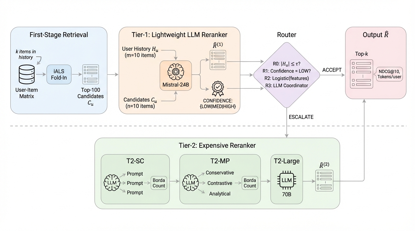
Figure 1: CascadeRec architecture: every request gets a cheap Tier-1 pass; the router uses history length and Tier-1 confidence, among other signals, and may escalate to a more expensive Tier-2 (self-consistency, multi-path, or a larger model).
The production router is a zero-latency heuristic based on history length and Tier-1 confidence. Note that production did not copy the τ=5 setting used in the offline experiments (escalate when history has at most 5 items); the rule's escalation direction and threshold are configuration, not code.
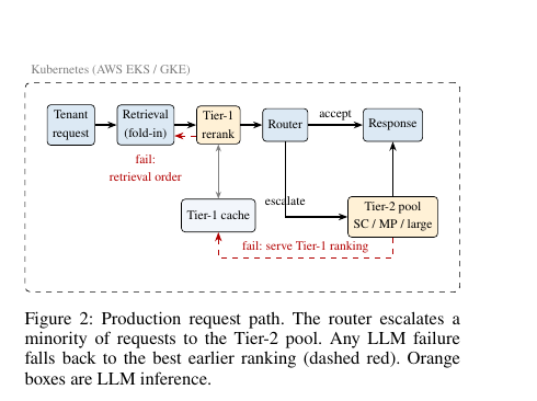
Figure 2: Production request path: retrieval, Tier-1, the router, and an optional Tier-2 pool; any LLM failure falls back to the best earlier ranking (dashed red).
Production A/B
The experiment has run for more than a month. The control group is the previous uniform expensive reranking; the treatment group is CascadeRec. Tier-1 results are cached per (user, model, seed), and every downstream consumer, including the control group, reads the same Tier-1 ranking. "Exactly comparable" holds only at the level of this key: for the same user, model, and seed, both groups get the same Tier-1 ranking, so differences between the groups do not come from Tier-1 sampling noise. The authors say this removed a class of spurious regressions caused by sampling noise and lets online A/B and offline replays be checked against each other. Results and their scope:
- Cost: the treatment group's inference cost is about 10% lower, measured by token accounting. This is an overall comparison of the two groups. The treatment group includes every change shipped together with the cascade, so the saving is not attributable to the routing policy alone.
- Quality: no regression has been observed so far. The authors report parity and do not claim a gain. Because business metrics are still accruing, the result so far is parity only; effect sizes await the final A/B readout.
- Latency: the impact is described as minimal, and non-escalated requests are essentially unaffected. This is a qualitative description.
Production uses only zero-shot models, and there has been no production comparison against per-tenant fine-tuned rankers.
4. Findings on public data
Tenant data cannot be released, so the authors run a reproducible offline evaluation on MovieLens-1M and Amazon-Electronics (2023). Key elements of the setup:
- For each user, one interaction is held out as the evaluation target, and the history is truncated to the k most recent items before that interaction, with k∈{1,3,5,10,20} and 200 users per bin.
- Retrieval uses implicit ALS (alternating least squares) with fold-in. The retriever sees only the truncated history, but its latent space is trained on the full population; the authors state explicitly that this is a deliberately strong baseline (B0).
- On MovieLens, the LLM reranks only the first 10 of the retrieved top-100. Positions 11–100 are outside the reranker's reach, and retriever Recall@100 is the ceiling; B0 is the retrieval order. On Amazon, the candidates are the held-out target plus 19 sampled negatives, 20 in total, ordered by retriever score; that order is B0, and the LLM reranks all 20. Each bin's score in the tables is based on that bin's 200 users. Because the protocols differ, Amazon's absolute numbers should be read as comparisons under a fixed protocol and should not be compared directly with MovieLens.
- The models are Mistral-Small-24B and Qwen3.5-27B, both zero-shot; the metric is NDCG@10. A star in the tables means the 95% interval of the delta versus B0, under a 10^4-resample paired bootstrap, excludes zero, which means that delta is statistically significant.
- The offline cascade uses τ=5, so bins with k≤5 are escalated; k=10 and k=20 are not escalated, and their results are bit-identical to uniform reranking B1. B1 is an offline baseline: every user is reranked once by the same zero-shot LLM, with no escalation. It is different from the previous uniform expensive reranking policy used by the control group in the production A/B.
Table 1: NDCG@10 by cold-start bin (200 users per bin; numbers from Table 1 of the paper). * means the 95% paired-bootstrap interval of the delta versus B0 excludes zero. The cascade, CascadeRec (CR in the table), uses τ=5, so bins with k≤5 are escalated.
| Dataset | Model | Method | k=1 | k=3 | k=5 | k=10 | k=20 |
|---|---|---|---|---|---|---|---|
| MovieLens-1M | – | B0 | .059 | .076 | .074 | .071 | .038 |
| Mistral | B1 | .053 | .070 | .066 | .070 | .048* | |
| Mistral | CR+SC | .054 | .066 | .069 | .070 | .048* | |
| Mistral | CR+MP | .053 | .074 | .071 | .070 | .048* | |
| Qwen | B1 | .061 | .070 | .073 | .069 | .041 | |
| Qwen | CR+SC | .059 | .062* | .076 | .069 | .041 | |
| Qwen | CR+MP | .056 | .063 | .077 | .069 | .041 | |
| Amazon-Elec. | – | B0 | .507 | .534 | .542 | .562 | .545 |
| Mistral | B1 | .356* | .471* | .479* | .495* | .513 | |
| Mistral | CR+SC | .337* | .462* | .443* | .495* | .513 | |
| Mistral | CR+MP | .340* | .448* | .450* | .495* | .513 | |
| Qwen | B1 | .410* | .511 | .525 | .504* | .551 | |
| Qwen | CR+SC | .419* | .513 | .537 | .504* | .551 | |
| Qwen | CR+MP | .408* | .520 | .532 | .504* | .551 |
Main findings:
- Uniform reranking harms sparse-history users. On Amazon + Mistral at k=1, B1 is 0.356* and B0 is 0.507, a relative drop of 29.8%, which is the "up to about 30%" cited in the abstract. In the same setting, Qwen's B1 is 0.410*, a drop of about 19%.
- Escalating cold users can be worse. On Amazon + Mistral at k=1, the cascade with self-consistency scores 0.337*, below uniform reranking's 0.356*. With Qwen, the cascade with self-consistency scores 0.419* against B1's 0.410*; escalation is roughly neutral, and both remain significantly below B0.
- The only significant gain appears in the longest-history segment. On MovieLens + Mistral at k=20, B1 is 0.048* and B0 is 0.038, about +27%. The authors note that the truncation in this bin favors recent behavior, which may not match the final click and may therefore depress the collaborative filtering baseline, so they ask for a cautious reading of this result.
- In aggregate, no LLM configuration beats B0. On the cost side, τ=5 yields an escalation rate of about 60%, and spends 40%–50% fewer Tier-2 tokens than escalating every request.
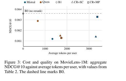
Figure 3: Aggregate trade-off on MovieLens-1M: average tokens per user versus NDCG@10. The dashed line is retrieval-only B0; both uniform reranking and the cascade spend tokens, yet stay below that line in aggregate.
Which offline segments benefit from escalation depends on the domain. So production does not copy τ=5. The production rule is set from per-segment deltas measured on tenant traffic. Traffic is segmented by history length and tenant size. Quality is compared between the treatment and control groups segment by segment, not only in aggregate. These deltas compare the two groups; they do not isolate the effect of Tier-2 or of extra inference. The rule changes only after a segment clears the rollout gate, and the gate checks exactly these per-segment deltas; full rollout proceeds tenant cohort by cohort, each opening once it clears its own gate.
5. Mechanism
The authors attribute the harm under sparse history mainly to a lack of preference evidence in the prompt. With only one or two history items, the model has very little user information to read; the authors' reading is that more samples or more diverse reasoning tend to reach the same wrong conclusion again. This is the authors' attribution, an interpretation of the experimental results.
6. Deployment lessons
- Measure segments first, then allocate compute. "Give harder requests more compute" does not hold here: cold users look hardest, yet escalating them can make results worse. The direction of escalation should be decided from measurements per segment and per domain.
- Offline thresholds do not transfer directly to production. τ=5 is an experimental setting used to test the intuition that cold users should always be escalated. Production did not copy it; the online rule's direction and threshold are configuration, adjusted from measured per-segment deltas.
- Read the cost and quality claims on their own terms. The ~10% is a saving for the treatment group as a whole, not the contribution of routing alone; quality parity means "no observed regression," not a demonstrated gain; the offline 40%–50% Tier-2 token saving is the routing effect isolated in a controlled setting.
- Build fallback into the request path. Offline parse-failure rates reach about 10% with a constrained prompt (10.4% for Qwen on MovieLens in Table 4), and Qwen's initial free-form output failed on 96.9%; falling back to the best available ranking ensures users never see an LLM error.
The core message of the paper: expensive inference should be allocated after measuring by segment, not added by default to every request or to every "hard" request.
How did this read for you?
Hoot made a note. Thanks for the feedback.

One tap, no sign-in; tap again to undo. Only anonymous counts are kept, never who you are.
Discussion
Add experiment details, reproduction notes or a different take. Requires a GitHub sign-in.
Loading the discussion…