Contents · 9 sections
1What problem is it actually solving?2Overall structure: per-day history, shared convolutions, set attention3The per-day history representation: letting the model see "how many days have passed"4Multi-scale convolution: reading rhythms from the 0/1 sequence5Set attention: candidate items consulting each other6Experiments: public data, ablations and internal data7Limitations as I see them8How a repurchase recommendation team could try it9VerdictSHARE

Teams building grocery and household "buy again" recommendations should read this paper, CASE (Cadence-Aware Set Encoding), because it points out a structural flaw in most repurchase models and offers a fix that can run as batch inference over tens of millions of users. The core idea in one line: represent each item's purchase history by "which day it was bought" rather than "which shopping trip", learn repurchase rhythms with multi-scale convolutions shared across all users, then let candidate items consult each other through a compute-saving form of set attention. On Walmart's large-scale internal data, its offline Precision@5 is 8.63% higher and Recall@5 9.90% higher than the production ranking model; on 3,744 Instacart test users, inference takes 19 seconds versus 318 seconds for the strong TIFUKNN baseline.
What problem is it actually solving?
Start with an illustrative scenario. Xiao Wang buys milk once a week and laundry detergent once a month. He last bought milk 6 days ago and detergent 10 days ago. What should we recommend today? Clearly milk is nearly due and detergent is not. Recommend too early and the suggestion feels irrelevant; too late and he may have already bought it elsewhere.
The paper tackles Next Basket Repurchase Recommendation (NBRR): rank only items the user has bought before, predicting which ones the next shopping trip will include again. The trouble is that most neural methods represent history as a sequence like "basket 1, basket 2, basket 3", where time appears only as basket order. So three trips on days 1, 8 and 36 look exactly the same to the model as three trips on days 1, 2 and 3; and predictions only change when a new purchase happens, so scores stay frozen during the days between purchases and cannot reflect "is this item due for restocking".
Another strong family is the neighbor-based TIFUKNN: compute time-decayed item vectors for each user, find similar users and aggregate their purchases. It works well, but every inference compares against the whole user base, which becomes infeasible at tens of millions of users. Some prior work already uses a per-day representation, but either has one set of convolution parameters per user, which does not scale, or does not extract multi-scale rhythms at the item level.
Overall structure: per-day history, shared convolutions, set attention
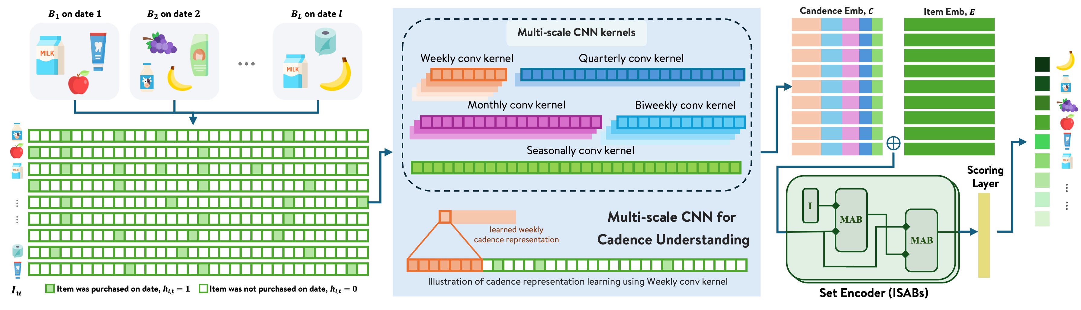
| Component | Input | What it does | Output |
|---|---|---|---|
| Per-day history | Purchase dates of each item the user bought | Over the last T days, mark 1 on days bought and 0 otherwise | One 0/1 sequence of length T per item |
| Multi-scale convolution | 0/1 sequence | Convolutions at five window widths, parameters shared by all users | Cadence vector (128-d) |
| Set encoding | Cadence vector concatenated with item embedding (128-d) | Two ISAB layers that let candidate items consult each other | Per-item representation (256-d) |
| Scoring | Two-layer MLP | Repurchase score, ranked by score |
The model has no "one per user" parameters at all, so it does not grow with more users, which is the precondition for batch inference.
The per-day history representation: letting the model see "how many days have passed"
Why switch? With basket-order representation, the time gaps are erased; with per-day representation, the gaps are written directly into the sequence. The window rolls, so each day the whole sequence shifts forward one cell, and even without a new purchase the model can produce a new ranking for the same user. This lets scores update daily between purchases, which is exactly what online restocking reminders need. The paper does not say on which day this training window of the calendar-time history representation ends (the last historical purchase or the day of the target basket), nor how the window aligns with the current day at inference. My reading is that ending the training window the day before the target basket, with the empty days in between included in the input, is what matches what the model sees when refreshed daily online.
How does it work? For each item the user has bought, build a -dimensional 0/1 vector , set to 1 on day if bought. The paper writes it only as a rolling -day window; the largest convolution window is 182 days, so must be at least half a year.
On the two public datasets without real dates (Instacart and DC (a dataset built from retailer Dunnhumby's public transaction data)), the authors reconstruct relative dates from fields like "days since prior order" and then build this sequence; TaFeng and the internal data keep real timestamps.
Multi-scale convolution: reading rhythms from the 0/1 sequence
How does it work? Apply one-dimensional convolutions of five widths over : weekly (7 days), biweekly (14 days), monthly (28 days), quarterly (91 days) and half-year trend (182 days). Each convolution's stride equals its window width, i.e. the sequence is cut into non-overlapping segments with one output per segment, so each scale gives activations. The activations from the five scales are concatenated and passed through two fully connected layers with ReLU to get the 128-d cadence vector .
Here is an illustrative example: assume days (a value I chose), then the segment counts per scale are: weekly 52, biweekly 26, monthly 13, quarterly 4, half-year 2, 97 positions in total. Xiao Wang's milk is bought weekly, so nearly every one of the 52 weekly segments has a purchase; detergent is bought monthly, so on the weekly scale only about one in every 4 segments lights up, while on the monthly scale every segment does. The two items "light up" differently across scales, which the fully connected layers use to separate "short-cycle" from "long-cycle" items, and whether the last few segments have already lit up shows how long it has been since the last purchase.
Why share parameters? The convolution kernels are the same set for all users and items, so they learn population-level patterns like "weekly buyers" and "monthly buyers" rather than one person's habits. A new user can benefit from these patterns as soon as there are a few purchases, and the parameter count is independent of the number of users. Earlier methods that learned per-user kernels see parameters explode at scale.
Set attention: candidate items consulting each other
Why is it needed? A user's candidate items form an unordered set, not a sequence. Yet items are related: someone who buys pasta often buys tomato sauce, and their restocking times corroborate each other.
How does it work? It uses ISAB (Induced Set Attention Block) from the Set Transformer. Ordinary self-attention makes items interact pairwise, with complexity. ISAB introduces learnable "induced points": first these points look at all items to form summaries; then each item looks back at the summaries. Complexity drops to . The paper uses two ISAB layers with and 4 attention heads.
Here is another illustrative example: a user has 200 previously bought items. Ordinary self-attention computes 200×200=40,000 pairs; ISAB computes 200×32=6,400 pairs in each of its two steps, 12,800 in total, about a third of the former. The more items, the more it saves.
Training uses binary cross-entropy: among the user's history items, those appearing in the next basket are positives and those that do not are negatives. Other hyperparameters: Adam, learning rate , batch 64, 30 epochs, dropout 0.1 after the ISAB layers and in the scorer.
Experiments: public data, ablations and internal data
The four grocery datasets cover different sparsity levels:
| Dataset | Users | Items | Baskets per user | Items per basket |
|---|---|---|---|---|
| Instacart | 18,739 | 37,522 | 16.7 | 10.07 |
| TaFeng | 7,227 | 18,703 | 7.52 | 6.58 |
| DC | 123,935 | 852 | — | 1.60 |
| Internal data | 10,308 | 88,812 | 43 | 11.72 |
Evaluation splits train and test by user, uses each user's last basket as the target, and restricts candidates to items the user bought before. There are five baselines: PersonalTop, ranking by historical purchase count; the neighbor method TIFUKNN; DNNTSP (graph aggregation over an item co-occurrence graph, then time attention by basket order) and BERT4NBR (BERT4Rec adapted to the next-basket setting), both modeling by basket order; and the authors' earlier PIETSP (set aggregation over item histories by time step, but without multi-scale rhythm extraction).
Below, Precision@1 and NDCG@10 compare CASE with the strongest baseline on each dataset:
| Dataset | Metric | Strongest baseline | CASE | Relative lift |
|---|---|---|---|---|
| TaFeng | Precision@1 | PIETSP 0.2507 | 0.2897 | +15.6% |
| TaFeng | NDCG@10 | PIETSP 0.3801 | 0.4021 | +5.8% |
| DC | Precision@1 | PIETSP 0.3886 | 0.3904 | +0.5% |
| Instacart | Precision@1 | TIFUKNN 0.5489 | 0.5478 | −0.2% |
| Instacart | NDCG@10 | TIFUKNN 0.5189 | 0.5241 | +1.0% |
| Internal data | NDCG@10 | TIFUKNN 0.3543 | 0.3514 | −0.8% |
This shows CASE's advantage concentrates on sparse TaFeng; the authors explain that with few purchases, neighbor aggregation is unreliable while the per-day rhythm signal is steadier. On the history-rich Instacart and internal data, it roughly ties TIFUKNN and is slightly lower on a few metrics. DNNTSP and BERT4NBR, which model basket order, generally lag on DC, Instacart and internal data, sometimes even below PersonalTop, which only ranks by purchase count. This shows representing time by basket order is a structural weakness that a more complex model cannot make up for.
CASE's real selling point is "tying TIFUKNN while being deployable". In inference complexity, CASE is per user, independent of the total number of users; TIFUKNN compares against all users per query, . Measured on 3,744 Instacart test users, CASE takes 19 seconds and TIFUKNN 318 seconds, about 17×.
The ablations are on Instacart:
| Model | Precision@1 | NDCG@10 |
|---|---|---|
| Full CASE | 0.5478 | 0.5241 |
| Without multi-scale convolution | 0.3333 | 0.3297 |
| Without set encoding | 0.5232 | 0.5152 |
| Without item embedding | 0.5390 | 0.5161 |
| Set encoding replaced by mean pooling | 0.5414 | 0.5225 |
Without the convolutions, Precision@1 falls from 0.5478 to 0.3333, below PersonalTop's 0.5019. This shows the per-day rhythm is the model's main signal source, with the other components adding to it; without time information, item embeddings plus set attention cannot even beat "rank by count". Removing item embeddings costs only 0.009, which shows deployment need not rely on huge, frequently refreshed embedding tables, good news for businesses with a growing catalog. ISAB is slightly better than mean pooling, but the gap is small.
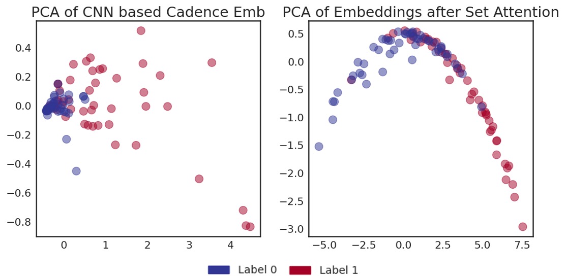
The authors use Figure 2 to argue that the convolutions already separate positives and negatives by rhythm, and set attention sharpens the boundary. This is just a 2-D projection of 100 points, good for a rough impression only.
Finally, the internal comparison, against Walmart's production ranking model with hand-engineered repurchase features, using the same candidate pipeline and data scale:
| K | Precision@K | Recall@K | NDCG@K |
|---|---|---|---|
| 5 | +8.63% | +9.90% | +10.46% |
| 10 | +6.78% | +7.95% | +9.40% |
| 20 | +5.27% | +6.32% | +8.75% |
This shows that at real scale, per-day rhythm modeling gives sizable gains over hand-engineered repurchase features, and the smaller K is, the larger the gain, which matters more for slots with limited positions.
Limitations as I see them
First, there is no online A/B yet. Table 3 is an offline relative lift, and the authors themselves say an online experiment is planned. Whether the offline gains turn into clicks and purchases has no evidence yet.
Second, the quality edge over TIFUKNN is small. On Instacart and the internal data, the two datasets closest to real business, CASE and TIFUKNN trade wins, with gaps around 1%. Its real value is inference cost, and 19 versus 318 seconds is a single measurement that depends heavily on implementation.
Third, several things must be decided yourself when reproducing, such as the window length and the number of convolution channels per scale; the source denotes the window only by the symbol , and channel counts do not appear. Only previously bought items are ranked, so new items and first purchases are outside the model's scope; the authors also admit that disrupted rhythms (e.g. buying through another channel, changing routines) have not been specifically studied.
How a repurchase recommendation team could try it
- First confirm repurchase share is high enough in your business. This direction is only worth it if most items in the next basket were bought before.
- Change your existing basket-order history into per-day 0/1 sequences with a window of at least half a year, add only the multi-scale convolutions and a simple scoring layer first, and compare offline against your current model. The ablations show this step captures the bulk.
- Then add set encoding. Start with mean pooling, then switch to ISAB, and see whether the gain is worth the extra complexity.
- Run daily-refreshed batch inference online, focusing on "whether items due for restocking rank near the top on the right days", e.g. hit rate bucketed by days since last purchase.
- Use small-slot metrics like Precision@5 as the offline gate for the online A/B, then look at actual clicks and purchases.
Verdict
For repurchase recommendation, changing time from "which basket" to "which day" matters more than switching to a more complex sequence model.
| Dimension | Assessment |
|---|---|
| Importance of the problem | High. Many items in grocery and household next baskets are repurchases, and timing decides the experience |
| Novelty of the method | Medium. Per-day representation, multi-scale convolution and ISAB all have prior work; what is new is combining them while keeping all parameters shared |
| Experimental evidence | Medium. Four datasets plus ablations with clear conclusions; but the edge over the strongest baseline is small and internal results are offline only |
| Engineering cost | Low. Small model, no per-user parameters, inference independent of total users |
| Worth trying? | Teams with high repurchase share whose current models represent time by basket order should first try the multi-scale convolution step |
How did this read for you?
Hoot made a note. Thanks for the feedback.

One tap, no sign-in; tap again to undo. Only anonymous counts are kept, never who you are.
Related papersMore from Paper Daily
 Personalization · 2026-09-02SetMIR: Multi-Interest Retrieval as Set PredictionDeep dive: SetMIR: Multi-Interest Retrieval as Set Prediction.
 Personalization · 2026-10-29Meta Andromeda: Powering the Next Generation of Ads Retrieval Through Model-System Co-DesignMeta's next-generation ads retrieval engine Andromeda brings near-ranking-quality models to retrieval, scoring every eligible ad. The new version replaces the single user tower with several specialized user towers as experts, and encodes the ad tower with real-time request context. An attention-based gate in the interaction layer activates only the most relevant experts per ad, cutting inference…
 Personalization · 2026-10-29Rethinking Positional Encoding and Interaction Granularity for CTR PredictionIn unified Transformer CTR models like OneTrans, the authors tried six positional encodings on Kuaishou's KuaiRand data, and none beat using no positional encoding at all. Building on this, the Wuhan University and Tencent paper proposes TRIP (the authors' name for the whole method). Each behavior encodes both its rank in the sequence and how long before this prediction it happened. Behaviors are…
Discussion
Add experiment details, reproduction notes or a different take. Requires a GitHub sign-in.
Loading the discussion…