SHARE

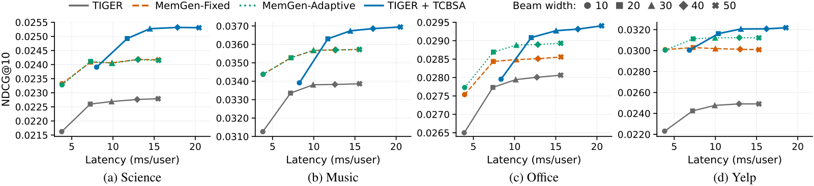
In generative recommendation with semantic IDs, the model writes an item's code one token at a time, and beam search keeps only the highest-scoring prefixes at each step. Once a prefix is pruned, every item beneath it can never be generated. The problem is sharpest when a user has just developed a new interest that shows up in only one or two recent interactions. Picture someone who has been buying phone accessories, has just bought a gaming mouse, and actually wants a mechanical keyboard next: the generator prunes the whole "gaming peripherals" branch at the first step. Give the same history to a model like SASRec that scores every catalog item directly, and the mechanical keyboard ranks second. This paper proposes TCBSA (test-time collaborative beam search adaptation), which turns the scoring model's item scores into bonuses on code prefixes before every pruning step, without retraining either model. On four public datasets, adding it to TIGER raises NDCG@10 by 4.9% to 30.4%; on all four datasets, TCBSA with beam width 20 is also more accurate than TIGER with beam width 50, with 23% to 32% lower latency.
Teams running generative retrieval should read this. It addresses a problem that is common in production but rarely handled on its own: generative models and conventional scoring models have different strengths, and the usual fix is to merge the two final lists, but items the generator pruned midway are already gone by the time you merge. The core idea in one sentence: the scoring model tells the generator which prefixes lead to good items, and the generator decodes as usual, adding that bonus before each ranking step.
What problem is it actually solving?
Walk through the example in the paper's Figure 1. Item codes have two levels (illustrative; the real experiments use four): at the first level, 42 means phone accessories and 81 means gaming peripherals; the second level identifies the item, so the mechanical keyboard is [81, 29] and the gaming mouse is [81, 14].
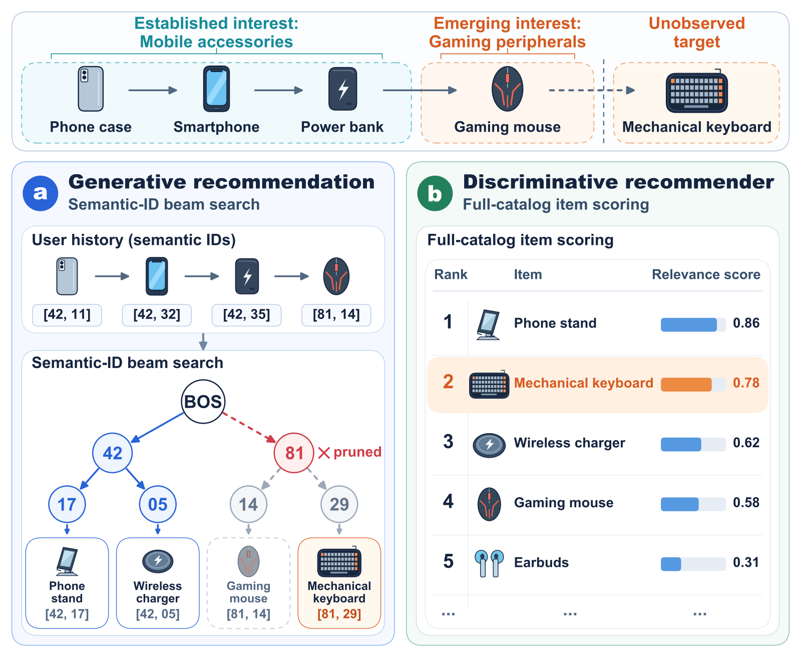
Three of the four history items are phone accessories and only the last one is a gaming mouse. The generator has learned that "this person buys phone accessories" and gives 42 a much higher probability than 81 at the first step. If the beam only has room for a few prefixes, 81 is pruned. Pruning is irreversible: the keyboard under 81 will never appear. The scoring model does not make token-by-token decisions; it scores every item directly, the most recent click on the gaming mouse weighs heavily, and the keyboard ranks near the top.
Why not just merge the two final lists? That is what the MemGen baseline does: each model produces a top-K, and the lists are mixed by weight. Merging can indeed pick the keyboard up from the scoring model's list, but only in the scoring model's order. Whatever the generator knows about the other items under the "gaming peripherals" branch is lost, because that branch was pruned at the first step. To let the generator itself walk down that branch, you have to step in before pruning.
The difficulty is that the two models speak different languages. The scoring model scores whole items; at each step the generator decides which token follows prefix 42, and many items hang under one prefix. So you need a way to translate item-level scores into prefix-level bonuses.
The big picture: one offline table, two online steps
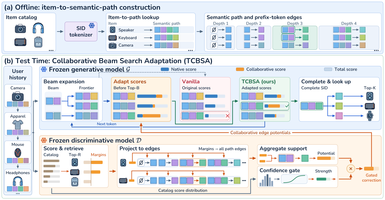
The pipeline:
- Offline: semantic IDs are fixed, so an item coded [c1, c2, c3, c4] maps to four edges: "empty prefix to c1", "prefix c1 to c2", and so on. Store these four edges for every item in a lookup table.
- Online step one: the scoring model scores the catalog, keeps the top R (R=500 in the experiments), spreads the margins onto edges to get a bonus per edge, and multiplies by a factor that reflects how confident the scoring model is.
- Online step two: the generator runs ordinary beam search, except that before each ranking step it adds the edge bonus to the path's cumulative score.
The key division of labour: the scoring model only signals whether good items lie down a path, and the generator still writes the code step by step. Neither model's parameters change. Now the pieces.
Step one: spread item scores onto code edges
Why not use the raw scores? Such scores have no natural zero point. Add 10 to every item and the ranking is unchanged, but adding raw scores to the generator's log-probabilities would shift results arbitrarily. So the authors only look at how far each item sits above the R-th item:
Here is the scoring model's score for item and is the R-th highest score. Items below rank R get zero, and the margin is unaffected by a uniform shift.
One edge may be passed by several top-R items. The edge "prefix 81 to 29" may be passed only by the keyboard, while "empty prefix to 81" is passed by the keyboard, the mouse, headsets and every other gaming peripheral. The margins of the items sharing an edge are combined into one number, the edge bonus , where is the current prefix and the candidate token. By default the bonus is the mean of the eight largest margins; on Yelp it is the maximum.
A small example you can do in your head (illustrative): in the top R, the keyboard is 0.9 above the R-th score and the mouse is 0.5 above it. Both pass "empty prefix to 81", so that edge gets their mean, 0.7. A phone stand is 0.3 above the cutoff and passes "empty prefix to 42", so that edge gets 0.3. Edges that no top-R item passes get 0.
A side effect: items outside the top R can benefit too. If an item shares part of its prefix with a top-R item, that shared part is protected, and the generator completes the remaining tokens on its own. This does happen in the experiments, as shown below.
Step two: scale the bonus by the scoring model's confidence
Why is this needed? The scoring model is sometimes unsure. Applying the same strength to every user means that for users where the scoring model has no idea, the bonus just scrambles an ordering the generator had right.
Confidence is measured cheaply: softmax the scoring model's catalog scores and take the largest probability . The more the scores concentrate on a few items, the larger is. A sigmoid then maps to a strength:
is the maximum strength, sets how sharp the switch is, is the threshold and is the sigmoid. Above the threshold the strength approaches ; below it, the strength drops quickly.
With the parameters chosen on the Science dataset, , , : a user with gets , a sigmoid of about 0.73, and a strength of about 0.87. A user with gets a sigmoid of about 0.27 and a strength of only about 0.33. The same edge bonus is applied at a bit over a third of the strength for the second user.
Step three: add the bonus to the path score before pruning
The generator's cumulative score for a path is the sum of the log-probabilities of its tokens. TCBSA adds one term to that sum:
is the existing cumulative score of prefix , is the generator's own log-probability for the next token, and is the bonus. At each step the top B are kept by this new score; the generator's output probabilities are untouched.
Continuing the example (illustrative): at the first step there are three candidate prefixes with log-probabilities 42: −0.5, 55: −1.2, 81: −1.6, and the beam keeps two. Without bonuses, 42 and 55 survive and 81 is pruned. With strength 0.87, 42 becomes −0.5+0.87×0.3≈−0.24, 55 has no bonus and stays at −1.2, and 81 becomes −1.6+0.87×0.7≈−0.99. Now 42 and 81 survive, and the keyboard's branch is saved. Hoot says

Rerank after pruning (baseline)
- prune by raw score
- 42 (−0.5), 55 (−1.2) survive
- 81 (−1.6)
- pruned at step one
- then add bonuses
- only orders 42 and 55
- the keyboard branch
- cannot come back
The whole subtree under a pruned prefix is never generated, so post-processing cannot reach it.
Bonus before pruning (TCBSA)
- 42
- −0.5 + 0.87 × 0.3 ≈ −0.24
- 55
- no bonus, still −1.2
- 81
- −1.6 + 0.87 × 0.7 ≈ −0.99 → survives
- check the survival rule
- 42 may be ignored; vs 55: 0.87 × 0.7 ≈ 0.61 > 1.6 − 1.2 = 0.4 ✓
The condition holds, so 81 ranks at worst 2nd and must stay in the beam, matching the direct computation above.
Uses the text's illustrative numbers (beam of 2, strength 0.87). The rerank-after-pruning column is our baseline; the last row on the right plugs these numbers into the appendix's survival condition. Source: paper §4.3: path score S(p⊕t) = S(p) + log π₀(t|p) + ηA(p,t), top B kept each step by the new score; appendix survival condition: at most B−1 may be ignored, every other one needs η × bonus gap > raw-score gap
The appendix gives a survival condition. Split the other candidate prefixes at the same depth into two groups: at most B−1 of them can be ignored, and every remaining one must satisfy "the extra bonus the target earns over it, multiplied by the strength, exceeds the target's deficit to it in the original score". Then all the remaining ones rank below the target, the target ranks at most B-th, and it stays in the beam. When the scoring model is unsure, the strength is pushed down and the change to the original ordering is bounded.
How the experiments were run
The data are three Amazon Reviews 2023 categories (Industrial and Scientific, Musical Instruments, Office Products, called Science, Music and Office below) plus Yelp. Each user's last interaction is the test item, the second-to-last is for validation, and inputs keep at most the 20 most recent interactions. Evaluation ranks the full catalog with no negative sampling. The generators are TIGER and MiniOneRec; item codes come from Sentence-T5 text embeddings quantized by three-level RQ-K-means plus one de-duplication token, four tokens in all. The scoring models are SASRec or GRU4Rec. Baselines include Human-Prior (behavioural priors added at training time), APAO-Pairwise (prefix-aware training) and two versions of MemGen (merging final lists). Default beam width is 20 and R=500. Hyperparameters are tuned only on the TIGER plus SASRec pair and reused unchanged for the other two pairs.
Does it actually work better?
Main results first. NDCG@10, copied from Table 1 of the paper:
| Method | Science | Music | Office | Yelp |
|---|---|---|---|---|
| TIGER | 0.0226 | 0.0334 | 0.0277 | 0.0242 |
| SASRec | 0.0198 | 0.0318 | 0.0215 | 0.0281 |
| MemGen-Adaptive (merges final lists) | 0.0241 | 0.0353 | 0.0287 | 0.0311 |
| TIGER + TCBSA(SASRec) | 0.0249 | 0.0363 | 0.0291 | 0.0316 |
| MiniOneRec | 0.0244 | 0.0326 | 0.0262 | 0.0365 |
| MiniOneRec + TCBSA(SASRec) | 0.0260 | 0.0350 | 0.0268 | 0.0400 |
The paper reports four metrics (Recall@5, Recall@10, NDCG@5, NDCG@10) on four datasets, 16 comparisons in all. Across these 16 dataset-metric combinations, the best result always comes from some TCBSA variant, and 14 are significantly better than the strongest baseline. On the same TIGER and SASRec pair it beats list-merging MemGen on every dataset and metric. Stepping in before pruning really does recover more than merging lists afterwards. With MiniOneRec the gains are smaller (NDCG@10 up 2.3% to 9.6%). My reading is that MiniOneRec has already been trained with reinforcement learning, its original beam is more accurate, and there is less to rescue.
Next, new interests. The authors cluster item text embeddings into 16 groups and pick users whose last one or two interactions fall in a new group while at least three of the four before them belong to another. On Science, among the 602 users with a single new-interest interaction, TIGER's NDCG@10 is 0.0398 and 0.0462 with TCBSA. That means it helps exactly where the generator is weakest. On the Yelp subset with a single new-interest interaction, though, SASRec alone is still best (0.0525 versus 0.0502); the scoring model is good at picking up the latest behaviour on its own.
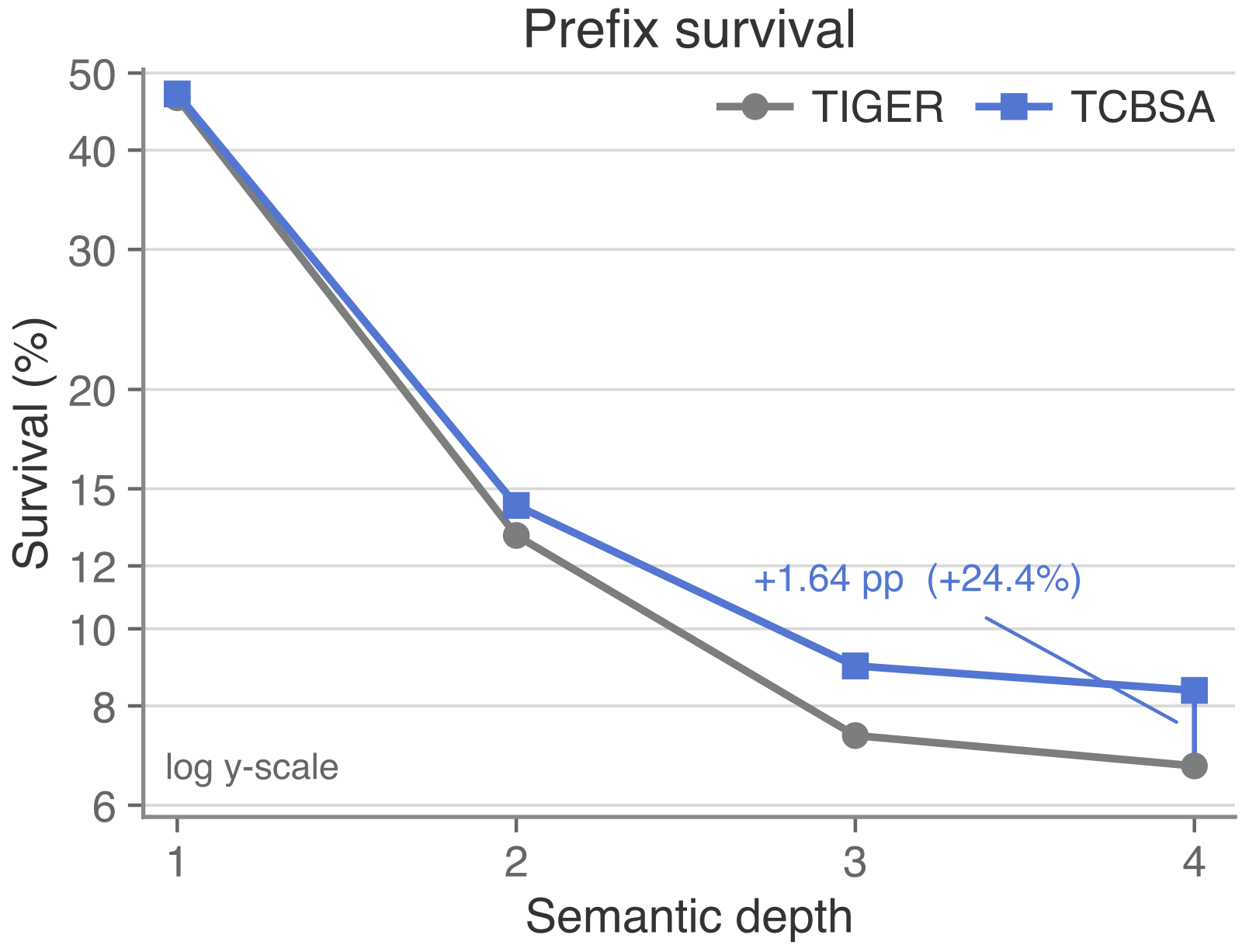
Does it really work by saving prefixes? The authors traced decoding on Yelp. At the last level, target-prefix survival rises from 6.72% to 8.37%. Of the 28,385 cases where plain TIGER first prunes the target prefix, TCBSA rescues 2,163 at the same step; 985 of them survive to the full code, and 632 end up in the top 10. The rescued tokens have a median rank of 22 in the generator's own ordering, and 56.68% sit outside its original top 20. So the bonus really does pull back branches the generator ranked poorly. There is a cost: it pushes out 12.68% of target prefixes that would have survived the first level, but total top-10 hits rise from 1,393 to 1,738, a net gain of 345.
Is the shared-prefix effect real? The authors ran an intervention: for items that are not in SASRec's top 500 yet were correctly recommended by TCBSA, they removed the bonus on that item's own code path and reran. On Office, 29.89% of the 532 such hits were lost; as a control, removing equally strong bonuses that are not on the target path lost only 0.04%. These hits genuinely come from the bonus of sharing a prefix with top-R items, not from coincidence.
Does the confidence gate matter? Removing it and using full strength for every user lowers NDCG@10 by 1.88% to 9.08%. The different ways of combining margins (mean, maximum and so on) differ by less than 2%, so the combination rule matters little and the gate is what counts.
Finally, latency. At the same beam width of 20, TCBSA takes 1.43 to 1.63 times as long as TIGER, because it adds one full-catalog pass of the scoring model. Compared with widening the beam, however, it is the better deal: TCBSA at beam 20 is more accurate than TIGER at beam 50 and still 22.95% to 32.27% faster, which shows that the extra scoring time costs less than more than doubling the beam. Recovering what pruning loses is cheaper with smarter ranking than with a wider beam.
Where I think it falls short
First, production has to run an extra full-catalog scoring pass. The paper measures latency on an RTX 5880 GPU with batches of 32 users, at 1.43 to 1.63 times the original for the same beam width. The largest catalog in the experiments is about 78 thousand items (Office). With millions to hundreds of millions of items, scoring the full catalog and taking the top 500 gets much more expensive and usually means switching to approximate retrieval; whether the bonus signal weakens then is something you have to measure on your own large catalog.
Second, the gain depends heavily on the gap between the scoring model and the generator. TIGER is weak on Yelp to begin with and gains 30.4% in NDCG@10; MiniOneRec on Office gains only 2.3%. If your generator is already far stronger than your scoring model, there is less signal to borrow.
Third, all experiments are offline on public datasets, and item codes have only four tokens. With deeper codes and more candidates per level, pruning happens more often, so TCBSA might gain more, or the bonus might be spread thinner and gain less. You will only know by running it on your own codes.
How a recommendation team could try it
- Diagnose offline first: on your current generative retrieval, log how many target prefixes survive at each level and see whether many are pruned in the first one or two levels. If survival is already high, there is nothing to rescue.
- Build a minimal TCBSA with an existing sequential scoring model (for example a SASRec-style retriever already in production): margins spread onto edges with a fixed strength, no confidence gate, and compare recall at the same beam width.
- If it helps, add the confidence gate. In the paper, removing the gate costs up to 9% NDCG@10, and its three parameters only need one sweep on a validation set.
- Measure latency last, against a beam widened to the same time budget rather than against the original beam. That is the comparison that matters for launch.
Bottom line
The pruning loss in generative recommendation can be recovered mid-decoding with an off-the-shelf scoring model and no model changes; the key is to step in before pruning, not after the lists are produced.
| Dimension | Assessment |
|---|---|
| Problem importance | High. Semantic-ID generative retrieval in production routinely loses items to beam pruning |
| Novelty | Medium-high. Spreading item scores onto code prefixes is simple, but it targets exactly where the two model types fail to connect |
| Evidence | Medium-high. Four datasets, three model pairings, decoding traces and intervention controls; all offline |
| Engineering cost | Medium. No training, but one extra full-catalog scoring pass; about 1.4 to 1.6 times the latency at the same beam width |
| Worth trying | Yes. Teams already running generative and conventional retrieval side by side can validate it offline in a few days |
How did this read for you?
Hoot made a note. Thanks for the feedback.

One tap, no sign-in; tap again to undo. Only anonymous counts are kept, never who you are.
Discussion
Add experiment details, reproduction notes or a different take. Requires a GitHub sign-in.
Loading the discussion…