SHARE

Most generative recommenders give every item a SID of the same length. Popular items keep paying for fine-grained codes, and shortening the codes squeezes the semantics of long-tail items. JevRec borrows a rule from natural language, where common words are short, and keeps one shared codebook for all items. It sorts items by training-set interaction count into groups; the more popular the group, the more trailing fine-grained codes it drops, while long-tail items keep their full description, plus one collision code that keeps every item unique. A separate output head first predicts the length and then the content is generated for that length, which reduces gradient conflict between the two objectives on one head. On three public Amazon datasets it beats the strongest baseline on all 12 metrics (Recall@5, Recall@10, NDCG@5 and NDCG@10 on each dataset), by 6.52% on average, and beats TIGER by 12.04% on average. Each training epoch takes about 16% less time than TIGER, and inference is faster too.
Teams building generative recommenders should read it, mainly because it turns SID length from a global hyperparameter into a property of each item. The ablations also separate where the gain comes from fairly cleanly: lengths assigned by frequency help, random lengths recover only a small part of the gain, and reversing the rule so popular items get long codes is worse still. The caveat is scale. The model has 4 layers with hidden size 128, each catalog has about 25k items, and most baseline numbers are copied from earlier papers. Whether it holds on catalogs with tens of millions of items and larger models is something you would need to test yourself.
What problem does it address?
A generative recommender produces the SID of the next item one token at a time. A common recipe uses residual quantization to cut an item's text vector into several levels of codes: the first levels are coarse categories, later levels add finer detail, and a final collision code separates items that still share a prefix. Nearly every method gives all items the same length, for example three semantic codes plus one collision code, four tokens in total.
The trouble is that interactions are very uneven. Here is an illustrative game store example:
| Item | Training interactions | Fixed-length scheme | Problem |
|---|---|---|---|
| A hit open-world game | 2,000 | 4 tokens | It costs 4 tokens every time it appears in a history or as a target, so its fine codes are paid for 2,000 times |
| A mid-popularity strategy game | 25 | 4 tokens | About right |
| A niche action game | 7 | 4 tokens | Its collaborative signal is weak, so it needs a richer content description, yet it gets the same 4 tokens as the hit |
Shortening every item to 3 tokens to save cost also compresses the long tail. Giving the long tail more description makes every item longer, and popular items cost even more. A fixed length ties "how much semantic detail the whole catalog needs" and "how much encoding cost the actual interactions incur" to a single number.
Natural language solved this long ago. Frequent words are short, like I and you; rare words are long, like international. Language did not shorten every word; it made frequent expressions cheap while keeping a rich vocabulary. JevRec applies the same idea to item codes.
Overall design
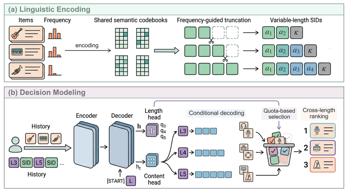
| Stage | What it does |
|---|---|
| Grouping | Sort items by training interactions and cut them into N groups, 3 by default, holding about 44.6%, 35.2% and 20.2% of items for high, mid and low frequency |
| Encoding | Encode item text with sentence-t5 and fit one 4-level residual quantizer shared by all groups; the high group keeps 2 levels, mid 3, low 4, each plus a collision code, for total lengths 3, 4 and 5 |
| Sequence format | Each item in the history is preceded by a length token that tells the model how many tokens belong to it |
| Length head | A three-layer network reads the history state and an embedding of each candidate length and outputs probabilities over the 3 lengths |
| Content head | The original T5 output layer, which generates codes after the length token |
| Inference | One beam search per length, slots allocated by length probability, then one ranking by length probability times content probability |
The model itself is small: 4 encoder and 4 decoder layers, hidden size 128, trained for 200 epochs on two H20 GPUs.
Mechanism 1: truncating codes by frequency
The key is that all items share one codebook. In residual quantization the early codes give the broad direction and later codes add detail on top, so dropping the last levels describes the same item at a coarser grain, without learning a separate semantic space for each frequency group.
The paper's case study shows the result for three games:
| Game | Training interactions | Group | SID | Length |
|---|---|---|---|---|
| Grand Theft Auto V | 2,142 | High | 36, 352, 1028 | 3 |
| Warcraft III: The Frozen Throne | 25 | Mid | 77, 412, 558, 1026 | 4 |
| Sekiro: Shadows Die Twice | 7 | Low | 23, 463, 514, 789, 1026 | 5 |
The last number in each SID is the collision code. After truncation several items in a group may share a prefix, and the collision code numbers them within the group so each full SID is unique. Collision codes can be reused across prefixes, since uniqueness is judged on the whole sequence.
Groups are cut by share of items, not by interaction thresholds. With a long tail, an absolute threshold such as "over 100 interactions is popular" would put most items in the longest group and leave the short groups nearly empty. The authors take a Gamma distribution with shape 2.1 and evaluate its density at the integers 1, 2 and 3, getting about 0.368, 0.290 and 0.167. Because those sum to about 0.825, normalizing gives 44.6%, 35.2% and 20.2%, which are the item shares of the three groups. The sorted list is then cut in that order. A smaller shape sends more items to the short groups. One setting is used on all three datasets.
Mechanism 2: predicting length and content separately
With variable lengths, the model must decide how many tokens the next item has before generating its codes. The direct option treats the length token as an ordinary token and lets one output layer predict it and then the codes. The authors argue the two tasks differ: length is a single three-way decision about the whole item, while content is token-by-token generation. Each training example has 1 length label but 3 to 5 content labels, so a shared head tilts training toward content.
They measured the gradient directions of the two objectives on shared parameters. At 27 checkpoints between epochs 5 and 135, they computed the cosine similarity between the length-loss and content-loss gradients over 48 batches each; a negative value means the two objectives pull in opposite directions.
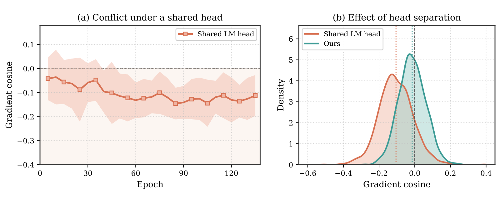
With a shared head the mean cosine is negative at every recorded checkpoint, and training does not bring the two back into agreement. With two heads the mean moves from -0.105 to -0.015. The conflict is much smaller but not gone, because both heads still sit on a shared backbone.
The length head concatenates the decoder's start state with the embedding of each candidate length, scores each pair with a three-layer network, and normalizes over the 3 legal lengths only. That length embedding is the same vector used as the prefix token when generating content, so what the length head picks matches the condition the content head receives.
Mechanism 3: slot quotas by length, then one ranking
If inference used only the most likely length, a wrong length guess would keep the correct item out of the list entirely. JevRec keeps every length branch and uses the length probabilities to decide how many slots each branch gets.
As an example, say the list has 10 slots and the length head gives probabilities 0.52, 0.31 and 0.17 (illustrative). Taking the integer parts of the proportional shares gives 5, 3 and 1, or 9 slots. The last slot goes to the length with the largest fractional part; 0.7 is the largest, so the length-5 branch gets one more, for a final 5, 3 and 2. Each branch runs its own beam search, keeps only codes that map to real items, and fills its quota by content probability.
The selected items are merged and ranked by length probability times content probability, so items of different lengths can interleave. If a branch cannot find enough valid items, its empty slots go to the best-scoring leftovers from other branches.
Results
The three datasets are Amazon Reviews 2023 categories: Musical Instruments, Industrial and Scientific, and Video Games, each with about 25k items and 50k to 95k users. Evaluation is leave-one-out over the full catalog with no negative sampling. Against the three strongest generative baselines (Recall@10 / NDCG@10):
| Method | Instrument | Scientific | Game |
|---|---|---|---|
| TIGER (fixed length) | 0.0564 / 0.0306 | 0.0422 / 0.0226 | 0.0868 / 0.0467 |
| LETTER | 0.0580 / 0.0313 | 0.0435 / 0.0232 | 0.0877 / 0.0473 |
| ActionPiece | 0.0615 / 0.0318 | 0.0452 / 0.0236 | 0.0927 / 0.0490 |
| JevRec | 0.0643 / 0.0340 | 0.0486 / 0.0253 | 0.0966 / 0.0514 |
The table shows only @10; in the paper's full table all 12 metrics at @5 and @10 beat the strongest baseline, with significance marked by a paired t-test. The relative Recall@5 gain is larger than the Recall@10 gain on every dataset, so the improvement concentrates at the top of the list.
The ablations matter most, because they say which part does the work:
| Variant | Versus JevRec | What it shows |
|---|---|---|
| Random lengths | 8.70% lower on average | Variable length alone is not the point; assigning it by frequency is |
| Long codes for popular items | Worse than random on every metric | The direction matters, supporting "popular short, long tail long" |
| Shared output head for length and content | 7.50% lower on average | Separate heads help |
| No length tokens | Largest drop in its group | The model must guess item boundaries and target length |
| History-only length head | Every metric within 1% of JevRec, relative | Separating the length decision matters; the exact scorer does not |
| No length quotas | All 12 metrics drop | Quotas keep the list consistent with the length distribution |
On efficiency, training time per epoch is 15.75% lower than TIGER on average, and total test-set inference time is lower on all three datasets. On Instruments, JevRec's validation NDCG@10 is above TIGER's at every checkpoint, and its best checkpoint arrives 20 epochs earlier.
The paper sweeps the number of groups N from 2 to 5 and the minimum length M from 2 to 5. For every N and for M from 2 to 4, NDCG@10 stays within 3.2% of the default. Once M goes above 3, NDCG@10 falls on all three datasets, most sharply from 4 to 5, because popular items are then forced into longer codes, which again supports the "popular items short" design.
Limitations as I see them
First, the scale is tiny. The model has 4 layers and hidden size 128, catalogs have about 25k items, and histories hold at most 20 items. Industrial generative recommenders usually have catalogs in the tens of millions, more code levels and much larger models. At that scale, nothing here tells us whether the tokens saved on popular items outweigh the extra error from length decisions.
Second, the comparison conditions are not fully matched. Most baseline numbers are copied from earlier papers, and the fixed-length ablation reuses TIGER's results rather than retraining JevRec's code with lengths fixed. Baselines use beam width 50, while JevRec uses 10 per length branch, 30 in total. These differences do not obviously favor either side, but they make it hard to say how much of the 6.52% comes from the encoding design and how much from implementation details.
Third, frequencies are computed once from the training set. New items have no interactions, popularity drifts, and once an item moves from the tail to the head its code length must change, along with what the model has learned about it. An offline leave-one-out evaluation never hits this problem; a live system always will.
How a generative recommendation team could try it
- Check your own distribution first: how much of the training interactions the top 20% of items account for, and the average token count of user histories under fixed-length SIDs. The more concentrated popularity is, the more frequency-based shortening saves.
- Run truncation directly on your existing residual-quantized codes, with no retraining of the quantizer: drop one level for the high group, keep one more for the low group, add per-group collision codes, and measure offline metrics.
- Run a random-length control at the same time. If frequency-based and random lengths look about the same, your gain likely comes from something else.
- Add a separate length head and compare it with treating the length token as an ordinary token. Log the cosine between the two loss gradients to see whether a shared head really shows persistent conflict in your setting.
- Plan for frequency drift before launch, for example regrouping weekly or letting items move only between adjacent lengths, and measure how re-encoding affects an existing model.
Bottom line
Assigning code length by interaction frequency, short for popular items and long for the tail, is the paper's most convincing finding: random lengths and reversed assignment are both worse, so the gain comes from matching frequency, not just from allowing variable length.
| Dimension | Verdict |
|---|---|
| Importance | Medium-high. Code length directly drives training cost and tail quality in generative recommendation |
| Novelty | Medium-high. Variable-length SIDs exist; frequency-grouped truncation with a shared codebook plus a separate length head is a new combination |
| Strength of evidence | Medium. Consistent gains on three datasets and clean ablations, but small scale and mostly copied baselines |
| Engineering cost | Low to medium. Encoding reuses an existing quantizer and the length head is a small network; drift is the hard part |
| Worth trying? | Yes, offline first: truncated codes plus a random-length control are cheap to test |
How did this read for you?
Hoot made a note. Thanks for the feedback.

One tap, no sign-in; tap again to undo. Only anonymous counts are kept, never who you are.
Discussion
Add experiment details, reproduction notes or a different take. Requires a GitHub sign-in.
Loading the discussion…