 CIKM 2026
SHARE

In HNSW graph indexes for vector search, once the vectors have been quantized, the edges of the graph often become the largest memory cost. This work from eBay and the University of Pisa shows that edges can be compressed losslessly to about half their size without slowing queries. It takes two steps. First, nodes are renumbered offline so that nodes that often appear in the same neighbor list get nearby IDs, which makes the differences between consecutive IDs in a list small. Second, those differences are stored in Stream VByte, a byte-aligned format that SIMD instructions can decode several integers at a time. On 7.26 million eBay product vectors, each edge shrinks from 33.3 to 18.3 bits, and mean query time at 98% accuracy falls from 632 to 564 microseconds. The method has run in eBay's search engine since early 2025, cutting graph memory by 44.3% with unchanged recall and latency.
Teams doing vector search, especially with quantized vectors, should read it. Its value is not a new algorithm but showing that the old search-engine recipe for inverted lists, renumber, store gaps, decode integers fast, also holds for HNSW, along with measurements of why other routes fail. One caution: the compressed index being faster than the original comes mostly from the memory locality that renumbering brings, not from compression itself.
Scenario
An illustrative scenario (not from the paper) shows why edges can dominate memory:
| Item | Unquantized | Vectors quantized with PQ |
|---|---|---|
| 10 million 96-dimensional vectors | 384 bytes each, about 3.8 GB | 48 bytes each, about 0.5 GB |
| About 50 edges per node, 32 bits each | about 2.0 GB | about 2.0 GB |
| Edges' share of the index | about a third | about 80% |
The harder you compress vectors, the larger the edges' share. In the paper's Figure 1, edges dominate both for eBay's 96-dimensional product vectors and for the PQ-quantized SnowFlake vectors.
Why edges are hard to compress
Each HNSW node links to at most 64 neighbors in the paper's setting, with forty to fifty on average. Each edge stores a neighbor's ID, and the default IDs follow insertion order, unrelated to graph structure. The authors measure the entropy of these IDs at 22.62 bits on eBay data, while storing each ID at fixed width costs only a little over 1 bit more. This shows IDs are nearly uniformly random, so fixed-width storage is already close to optimal and ordinary compression has nothing to work with.
The classic web-graph trick is reference copying: if one node's neighbor list resembles another's, record only which entries to copy. The authors compute the ideal savings: on the eBay graph a node has 49.9 edges on average but shares only 5.2 with its most similar node, so after paying to record which entries are copied, the whole graph saves at most 8.8%. The reason is that HNSW deliberately caps degree, so there are none of the hubs linked to thousands of nodes found in web graphs, and lists overlap little. That route is dropped.
Method: renumber, then store gaps
The second route is storing gaps. Sort a neighbor list and store only the difference between consecutive IDs. A hand example (illustrative): neighbors 1,203,881, 1,204,017, 5,330,102 and 5,330,250 need 23 bits each as raw values; as gaps they become 1,203,881, 136, 4,126,085 and 148, so small gaps need only 8 bits but large ones still need 22. Measured on the paper's data, gaps alone lower entropy from 22.62 to 18.52 bits, a small gain, because under default IDs neighbors are scattered across the whole ID range.
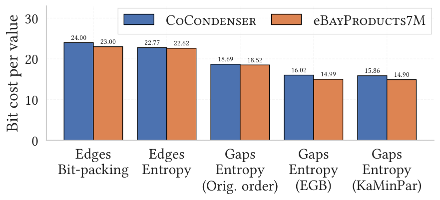
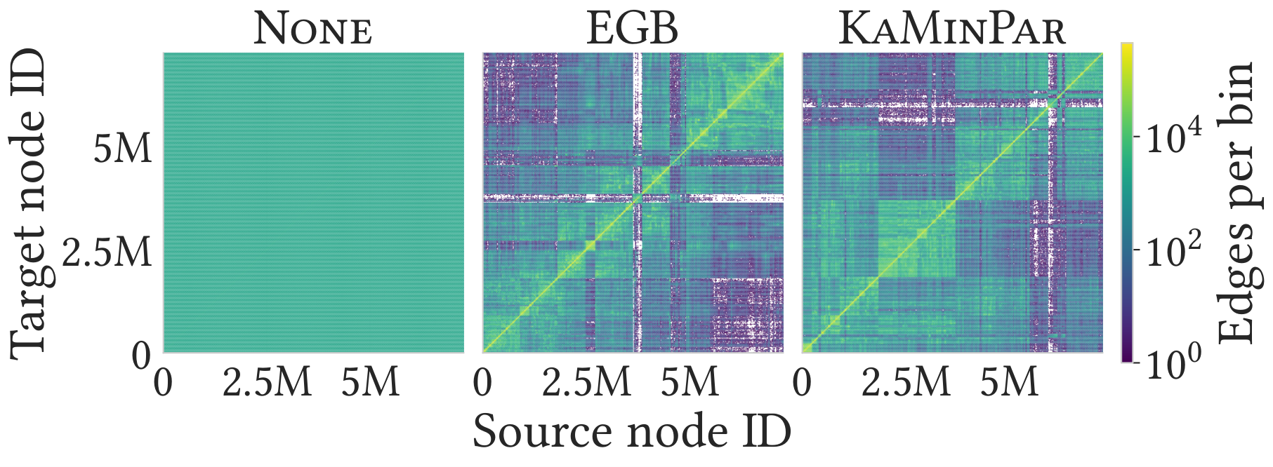
The key step is renumbering. The authors reassign IDs offline with EGB, a recursive bisection algorithm. It splits all nodes into two equal halves, then repeatedly swaps nodes between the halves, each time picking the swap that most lowers the total gap cost, until no swap helps. The cost is the estimated bits for gaps: for each neighbor list, count its neighbors in each half; with d1 of its neighbors in the left half of n1 nodes and d2 in the right half of n2, the cost is d1·log(n1/(d1+1)) + d2·log(n2/(d2+1)). The more neighbors in one half, the smaller their average spacing and the fewer bits each gap needs. After a swap, recomputing the affected lists gives the change in total cost. It then repeats this inside each half until blocks hold only a few nodes; the paper keeps the original algorithm's settings and gives no exact block size. Finally, nodes are numbered consecutively in partition order, so nodes in the same small block, which often appear together in neighbor lists, get nearby IDs. After reordering, gap entropy on eBay data falls further, from 18.52 to 14.99 bits.
Last comes the choice of format. Entropy is the floor, and integer formats differ in how close they get and how fast they decode. Zeta codes are the most compact but decode bit by bit, which is slow. Stream VByte stores each integer in 1 to 4 bytes and records each integer's length in 2 bits, packing four lengths into one control byte. Decoding then restores four integers with a single SIMD shuffle and no branches. It costs less than 1 bit per edge more than Zeta but decodes much faster.
Two small overheads remain. The array of list start positions, originally 64 bits per entry, is compressed with Elias-Fano to about 8 bits. And since results must be reported in original IDs, an inverse mapping must be stored after renumbering.
How decoding works at query time
Compression only matters if it does not slow queries, so the storage format must fit how HNSW reads data. An HNSW query walks the graph greedily: at each node it reads all neighbors, computes their distances to the query, and moves to closer ones. A query jumps to a few hundred nodes at random, each time needing one node's neighbor list.
So the authors compress per list, with each list as its own block starting at the position recorded in the start array. At a node, the query fetches the start from the Elias-Fano array and decodes only that block. A block holds forty to fifty gaps on average, which Stream VByte restores four at a time in a dozen or so SIMD instructions, followed by a prefix sum to turn gaps back into IDs. Computing distances to dozens of vectors afterwards costs far more, which is why latency barely changes.
A detail that is easy to miss: vectors are also stored in the new ID order, so neighbors with nearby IDs also sit near each other in memory, so caches and prefetching work better when vectors are read. That gain has nothing to do with compression, and it comes up again in the limitations.
Results
The authors compare four datasets with the same HNSW parameters, taking the fastest configuration at 98% accuracy, meaning the share of the true 10 nearest neighbors among the 10 returned:
| Dataset | Plain bits/edge | Stream VByte bits/edge | Zeta bits/edge | Plain time | Stream VByte time | Zeta time |
|---|---|---|---|---|---|---|
| eBay 7.26M products | 33.3 | 18.3 | 17.4 | 632 | 564 | 714 |
| CoCondenser 8.84M sparse | 33.4 | 19.4 | 18.7 | 778 | 765 | 819 |
| Sift 1M images | 34.1 | 16.1 | 14.6 | 111 | 114 | 141 |
| SnowFlake 8.84M PQ | 33.6 | 18.0 | 17.0 | 497 | 494 | 545 |
Times are in microseconds. This shows Stream VByte's space is only 4% to 10% above the most compact Zeta, while Zeta is about 27% slower on Sift. Stream VByte is no slower than plain on three datasets and only 3 microseconds slower on Sift.
Renumbering is a one-time offline cost, from 3.5% (CoCondenser) to 30% (Sift) of total index build time.
Limitations as I see them
First, "faster after compression" comes mostly from renumbering. The authors themselves find that renumbering alone, without compression, cuts plain query time by 3.0% to 17.0%, because nearby nodes also sit together in memory and caches hit more often. The plain baseline in the table uses default IDs. A fair comparison would be a renumbered plain index, against which Stream VByte would likely be slightly slower, but that column is absent from the table.
Second, the savings are on edges, not the whole index. On eBay data edges drop from 33.3 to 18.3 bits, about 45% saved, but if your vectors are unquantized and high-dimensional, such as 1024-dimensional floats, edges are a small share of the index and total memory falls only by single-digit percentages.
Third, only low-degree graphs with a cap of 64 are tested. The authors argue this is the harder case, but there is no data on gains or latency at higher degrees, and the code is not yet public; the authors say it will go into the kANNolo Rust library.
How a search team could try it
Step one: measure how much of your index is edges. Multiply average edges per node by 32 bits and compare with vector storage; if edges are under 30%, it is not worth the effort.
Step two: renumber only, without compression. That alone may speed queries by a few percent, and it needs only a one-time offline renumbering plus an inverse mapping.
Step three: add gaps and Stream VByte. Ready-made C and Rust implementations exist, the change sits in the function that reads neighbor lists, and before launch you should compare latency percentiles on your own query logs.
Verdict
In one sentence: HNSW edges look like random numbers, but after renumbering they compress as well as a search engine's inverted lists.
| Dimension | Assessment |
|---|---|
| Importance of the problem | Medium-high. With vector quantization widespread, edges become the main memory cost |
| Novelty of the method | Low to medium. Reordering, gaps and Stream VByte are existing techniques; the contribution is the combination and measurements |
| Experimental evidence | Medium. Four datasets plus production, but missing the renumbered-plain baseline |
| Engineering cost | Low. One offline reorder, and neighbor reads switch to decoding |
| Worth trying | Teams with quantized vectors and tight memory should try it directly; teams with unquantized vectors gain little |
How did this read for you?
Hoot made a note. Thanks for the feedback.

One tap, no sign-in; tap again to undo. Only anonymous counts are kept, never who you are.
Discussion
Add experiment details, reproduction notes or a different take. Requires a GitHub sign-in.
Loading the discussion…