SHARE

Teams that run generative recommendation on semantic IDs (SIDs) usually also own a strong conventional sequential model. The most reusable idea in REGER, a framework from the University of Electronic Science and Technology of China that explicitly models inter-item relations for generative recommendation, is to split that conventional model's scores onto every branch of the SID prefix tree. At each step the generator then learns not only which token is correct, but also how good the other branches are. Added alone to TIGER, this distillation lifts Recall@10 on Beauty from 0.0673 to 0.0794, raises training time per epoch from 19 to 23 seconds, and leaves inference time unchanged. Removing it from full REGER drops Recall@5 by 10.9% to 18.0% across three datasets, the largest effect of the three modules. The other two modules, a pretraining task that teaches which items have similar content and encoder attention heads that focus on adjacent interactions, are small changes that each add a few points. Keep in mind that all experiments use small Amazon datasets (Beauty has about 12 thousand items, histories truncated to 20), and with a poorly chosen teacher the top of the list gets worse.
What problem does it solve?
Generative recommendation encodes each item as an SID, coarse tokens first and fine tokens later, and generates the next item token by token. User preference and item similarity are defined on items, but the model's unit is the token, so inter-item relations must be inferred implicitly. The paper splits this into three gaps.
| Stage | Current practice | What is missing |
|---|---|---|
| Learning item semantics | Random token embeddings, model trained from scratch | Which items are similar in content |
| Encoding history | Concatenate history SIDs and run bidirectional attention | Explicit transition from the previous item to the current one |
| Generating the next item | Cross-entropy only marks the correct token | Cross-entropy does not directly teach the model to compare other candidates; the model learns these preferences implicitly |
An illustrative scenario runs through the piece: a beauty shopper bought a cleanser, a toner and a serum, and next buys a face cream. Each item has 4 tokens: skincare vs makeup, category, specific product, and a final token that separates items with identical codes.
Pipeline
| Stage | What happens | Gap addressed |
|---|---|---|
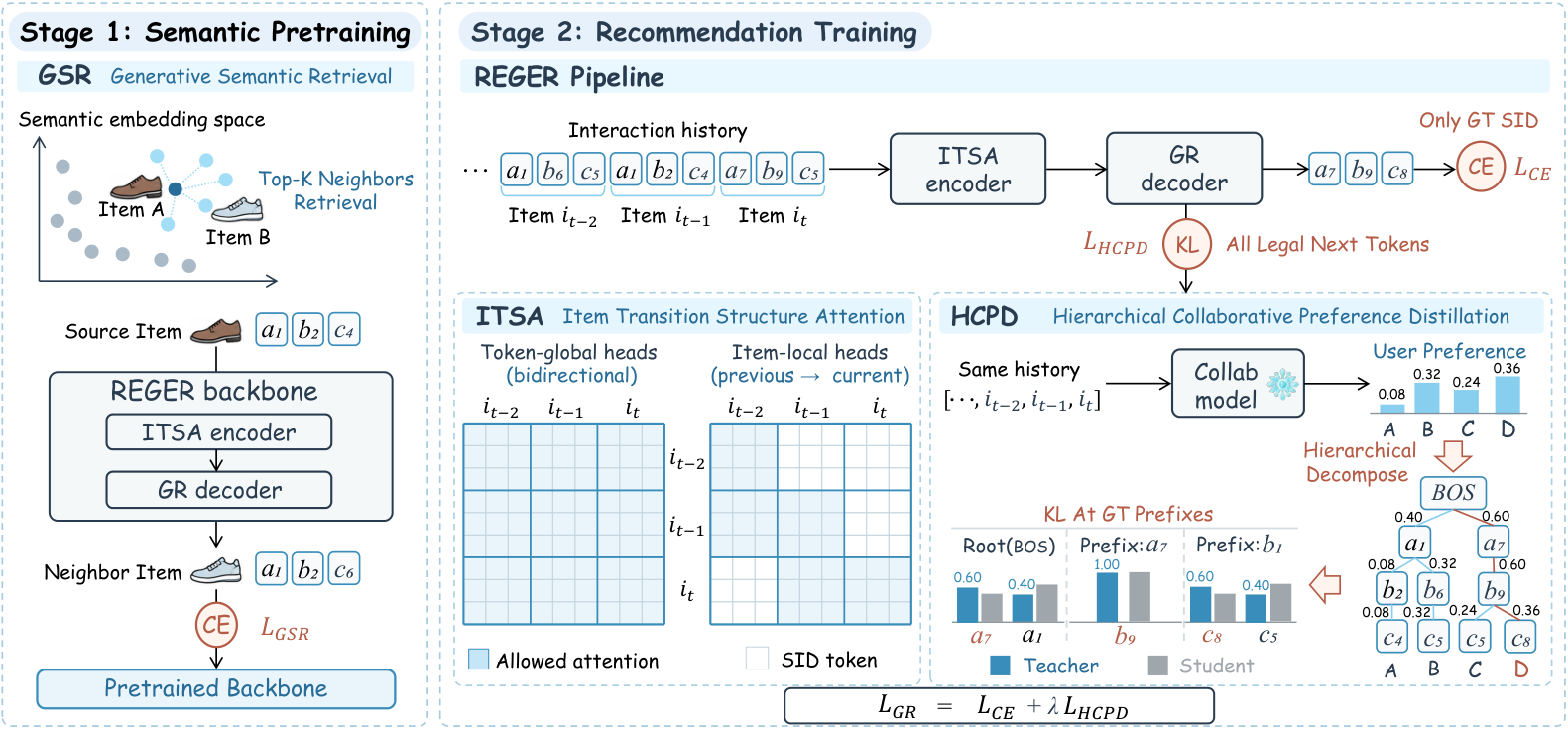
| Stage 1: semantic pretraining (GSR) | Given an item's SID, generate the SID of its most similar item by content | Item semantics |
| Stage 2: recommendation training | Encoder uses a new attention layout (ITSA); loss is cross-entropy plus preference distillation (HCPD) | History encoding and generation |
Inference is ordinary beam search as in TIGER, with no teacher and no extra module.
Semantic pretraining: learn who resembles whom
Why? A model trained from scratch has random token embeddings. Two face creams may share an SID prefix, yet the model does not know how similar they are until user behavior teaches it, and items with few interactions suffer most.
How? Using the text embeddings that feed the RQ-VAE tokenizer, find each item's 10 nearest neighbors by cosine similarity. Each pair of item i and neighbor j is a training example: the encoder reads i's SID and the decoder generates j's SID. No user behavior is involved.
Illustration: input the SID of one brand's moisturizing cream, generate the SID of another brand's repair cream. After many such pairs, the model uses cross-entropy to learn to generate neighboring items' SIDs, learning semantic relations between items in the process and the encoder learns to read an item's 4 tokens as one unit. The checkpoint is chosen by recommendation validation performance, not pretraining loss. Ten neighbors works best; 20 or 50 hurt, suggesting that distant neighbors teach unrelated items to look alike.
Encoder attention: look at "previous to current"
Why? The history is flattened into a long token sequence. In plain bidirectional attention every token sees every token, and the model must work out which tokens form one item and which items are adjacent. Yet a key signal in recommendation is the transition between consecutive interactions, such as buying a serum after a toner.
How? The 6 heads per encoder layer are split into two kinds by changing only the attention mask, with no new parameters.
| Head | What each token sees |
|---|---|
| Global head | Every token in the history |
| Local head | The 4 tokens of its own item plus the 4 tokens of the previous item |
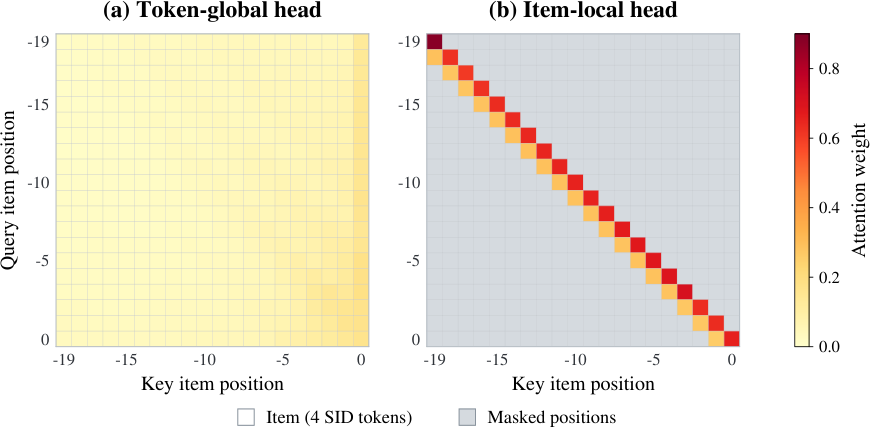
In the scenario the history has 12 tokens. In each layer's local head, the serum's tokens attend directly only to the serum and the toner; the toner's tokens attend directly only to the toner and the cleanser; the cleanser, being first, attends directly only to itself. Local heads can still receive earlier history indirectly: representations from the preceding layer can carry it, and global heads can bring it into each layer's output. Each local head is forced to answer one concrete question: what changed from the previous item to this one. Global heads supply longer-range context. The head ratio is tuned per dataset (local:global 2:4 on Beauty, 5:1 on Sports, 3:3 on Toys), and each beats all-local or all-global. Figure 4 shows a clear sub-diagonal band in the local head, confirming that it consistently attends to the previous item.
Preference distillation: split the teacher's scores across branches
This is the core of the paper and the largest gain.
Why? Cross-entropy uses only the true token as its target; it does not directly teach the model how to compare other candidates. But unchosen items are not equally bad: if a user bought a face cream, another face cream is probably a good recommendation and a lipstick is not. A conventional sequential model, DuoRec here, scores all items this way; the question is how to turn item-level scores into token-level supervision.
How? Three steps.
| Step | What happens |
|---|---|
| Teacher scores | DuoRec's parameters stay fixed. It reads the same user interaction history as the generator for the current example, scores every item, and applies softmax to obtain its preference probability for each item |
| Split by branch | At each prefix of the true target, sum the teacher's probabilities by which next token each item goes through, then normalize |
| Student matches | At the same prefix the student renormalizes its probabilities over branches that lead to real items, and minimizes the KL to the teacher's branch distribution |
The final loss is cross-entropy plus a weighted KL, with weights between 0.8 and 1.0 working best.
A hand-computable example with 4 items and 2 tokens each (illustrative): cream A (1,1) with teacher probability 0.4, cream B (1,2) with 0.1, lipstick C (2,1) with 0.3, lipstick D (2,2) with 0.2. The user actually bought cream B, path (1,2). At step 1 the teacher puts 0.5 on branch 1 (A plus B) and 0.5 on branch 2, so cross-entropy demands branch 1 while distillation says branch 2 is not bad either. At step 2, under prefix (1), A gets 0.4 / 0.5 = 0.8 and B gets 0.2. Cross-entropy demands token 2 (cream B), while distillation says that within this branch the teacher actually prefers A. Cross-entropy anchors the model to the real choice; distillation adds how good the other branches are. The KL gradient on each branch logit is proportional to student probability minus teacher probability, so an under-estimated branch is pushed up directly.
Why renormalize over real branches? Many vocabulary tokens map to no item under a given prefix. Comparing full-vocabulary probabilities to the teacher adds a penalty for insufficient legal mass that has nothing to do with the teacher and favors branches already likely. In the appendix, the full-vocabulary variant reaches NDCG@5 of 0.0382 on Beauty versus 0.0395 for the renormalized one.
The theory proves that an item's preference probability factorizes exactly into conditional probabilities along its SID path, and that item-level KL decomposes exactly into prefix-conditional KLs weighted by the teacher's prefix mass. Training only uses prefixes on the true path, so it approximates this full decomposition, and the authors spell out the difference.
Does it work?
Recall@10 on three Amazon 2014 datasets:
| Method | Beauty | Sports | Toys |
|---|---|---|---|
| DuoRec (discriminative, also the teacher) | 0.0875 | 0.0493 | 0.0961 |
| TIGER | 0.0673 | 0.0432 | 0.0659 |
| ActionPiece | 0.0772 | 0.0473 | 0.0729 |
| LIGER (generative plus dense retrieval) | 0.0830 | 0.0480 | 0.0838 |
| REGER | 0.0870 | 0.0545 | 0.0934 |
REGER beats every generative and hybrid method on all datasets and metrics. Against its teacher it is clearly better on Sports, about equal on Beauty, and lower in recall on Toys with equal or slightly better NDCG. The student absorbs the teacher's preferences while also using SIDs and semantic pretraining, and sometimes surpasses the teacher.
Distillation alone, with every method added to the same TIGER and DuoRec as teacher:
| Method | Beauty R@10 | Sports R@10 | Toys R@10 | Train s/epoch | Test s |
|---|---|---|---|---|---|
| TIGER | 0.0673 | 0.0432 | 0.0659 | 19 | 16 |
| + TCA-Aux | 0.0721 | 0.0455 | 0.0738 | 22 | 106 |
| + GFlowGR-TB | 0.0699 | 0.0436 | 0.0660 | 239 | 16 |
| + HCPD | 0.0794 | 0.0501 | 0.0823 | 23 | 16 |
Preference distillation (HCPD) is best while training is only a few seconds slower and inference unchanged. GFlowGR imposes flow-balance constraints on whole generation trajectories and trains more than ten times slower; TCA, which turns teacher scores into token soft labels, needs constrained decoding and multiplies test time. For production, unchanged inference with slightly longer training matters as much as the offline gain.
Ablation, Recall@5:
| Variant | Beauty | Sports | Toys |
|---|---|---|---|
| Without semantic pretraining | 0.0537 | 0.0346 | 0.0557 |
| Without local attention | 0.0566 | 0.0340 | 0.0579 |
| Without preference distillation | 0.0514 | 0.0318 | 0.0502 |
| Full REGER | 0.0594 | 0.0357 | 0.0612 |
In these ablations, Recall@5 drops most when preference distillation is removed, showing that it matters to the full model; the other two modules matter more on Beauty and Toys than on Sports.
Limitations
First, the data are small. Beauty has about 22 thousand users and 12 thousand items, with histories cut to 20. The teacher scores the whole catalog and applies a softmax; with millions of items this step must be sampled or restricted to candidates, so how much of the result survives needs checking.
Second, a weak teacher has side effects. With SASRec as teacher, Beauty Recall@5 falls from 0.0514 without distillation to 0.0465, while Recall@50 rises from 0.1685 to 0.1759. The KL pushes up good items the student under-rates but also copies the teacher's ranking errors, so long-list recall improves while the head gets worse.
Third, there are many knobs. The head ratio differs on every dataset, the distillation weight ranges from 0.8 to 1.0, and the pretraining checkpoint is picked by recommendation results, so moving to a new product carries real tuning cost.
How a recommendation team could try it
- Start with preference distillation. Use an existing retrieval or ranking sequence model as teacher; at each prefix of the true target, sum its probabilities by branch, normalize, and add a KL against the student's distribution over legal branches, sweeping the weight from 0.5 to 1.0.
- With a large catalog, let the teacher softmax only over its top few thousand candidates and set other branches to zero, then check that the gain holds.
- Before switching teachers, compare Recall@5 and Recall@50. If the long list improves but the head worsens, the teacher's ranking is not precise enough; use a stronger teacher or a lower weight.
- Then try local attention heads. They add no parameters; start with half local and half global.
- Leave semantic pretraining for last; it helps most where many items are cold, and the checkpoint should be chosen on recommendation validation.
Bottom line
A discriminative model's preference over all items can be split exactly into branch preferences along the SID prefix tree, and distilling those along the true path teaches a generative recommender how good the other candidates are at almost no inference cost.
| Dimension | Assessment |
|---|---|
| Importance | High. With cross-entropy alone, the training objective does not directly teach the model to compare candidates; the model learns these preferences implicitly |
| Novelty | Medium-high. Branch-level preference distillation is well grounded; pretraining and local attention combine familiar ideas |
| Evidence | Medium. Six public datasets, over ten baselines, training and inference cost; but only small academic data and no online test |
| Engineering cost | Low to medium. Inference unchanged, training slightly longer; full-catalog teacher scoring needs adaptation at scale |
| Worth trying | Yes, especially for teams with a strong sequential model moving to generative retrieval; try the distillation alone first |
How did this read for you?
Hoot made a note. Thanks for the feedback.

One tap, no sign-in; tap again to undo. Only anonymous counts are kept, never who you are.
Discussion
Add experiment details, reproduction notes or a different take. Requires a GitHub sign-in.
Loading the discussion…