SHARE

In an ad auto-bidding system, a PID (proportional-integral-derivative) controller adjusts bids every few seconds according to spend progress, but one set of controller parameters has to serve hundreds of thousands of campaigns with different budgets, lifetimes and traffic. Pinterest does not let reinforcement learning bid directly. Instead, each day it picks one of 9 parameter-multiplier combinations for each campaign, nudging the defaults one small step up or down, and PID keeps running as before. In a seven-day online A/B test, effective cost per click (eCPC) fell a significant 0.25% with revenue essentially unchanged; over two months after rollout, compared with holdout traffic, campaigns more than a week from their end had eCPC almost 1% lower.
Teams working on bidding and budget control should read this, mainly for the deployment pattern: reinforcement learning only decides "which parameters to use today", the result is written into a lookup table, no model is loaded at serving time, and the worst case is parameters one small step away from the defaults, so the safety boundary is very clear. But be clear about its limits. The discount factor is set to 0, so what is learned is really a contextual bandit that picks one action per day and looks only at that day's outcome. All cross-day trade-offs are left to a hand-designed weight curve. Online gains are only a few tenths of a percent, and the long-run post-rollout data has no significance test.
What problem is it solving?
PID controllers are the industry's most common budget-pacing tool. A PID controller watches the gap between actual spend progress and a target spend curve: the proportional term looks at the current gap, the integral term at the gap accumulated so far, and the larger the error, the harder the bid adjustment. The coefficients and set how strongly it reacts.
The problem is that no single set of coefficients suits every campaign. Take one campaign's lifetime as an illustration:
| Point in time (illustrative) | Campaign state | Better control style |
|---|---|---|
| Day 3, 7 days left | Unspent budget can roll over | React more gently, chase fewer expensive impressions to catch up, keep cost per click down |
| Day 9, 1 day left | Remaining budget expires after today | React more aggressively, prioritize spending the budget |
| A very large-budget campaign | High traffic demand, big swings | May need different strength from small-budget campaigns |
Fixed parameters can only compromise between these cases. The paper keeps PID but, every morning, picks a set of coefficients for each campaign based on its state.
Pipeline overview
| Component | What it does | Cadence |
|---|---|---|
| State | Campaign ID embedding, remaining days, daily budget, target spend curve, previous day's CTR, CPC and revenue | Daily |
| Action | Multiply each of and by one of , 1 or , giving 9 combinations; the derivative term stays fixed because its error signal is too noisy | Daily |
| Decision | A two-headed Q-network predicts each action's relative change in budget utilization and in CPC, then merges them weighted by remaining days | Once a day at midnight |
| Serving | Results are written into a campaign-to-parameters lookup table; the bidder reads it every few seconds and runs PID with those parameters | Seconds |
| Exploration | Each campaign sets aside a small share of budget and separate user buckets for random actions, to collect training data | Continuous |
The paper's example value of is 0.2, i.e. 20% above or below the default. The action space is deliberately tiny to keep online exploration close to a validated configuration.
Predict two objectives separately, merge them at serving time
Budget utilization and CPC naturally conflict: bid higher and the budget spends faster but each click costs more; bid lower and CPC looks good but the budget may go unspent. The usual approach combines both rewards into one weighted number before training, but then any change in weights requires retraining.
The paper puts two output heads on a shared network trunk, one predicting the change in budget utilization and one the change in CPC, each with its own training loss. They are merged only at inference:
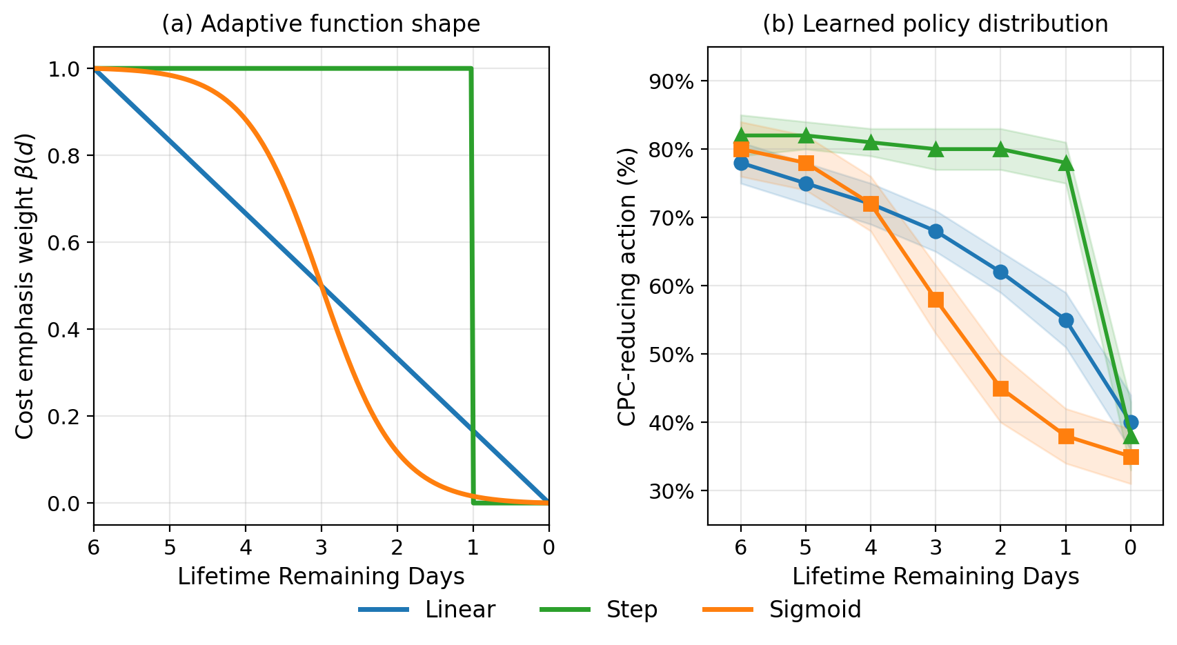
is the campaign's remaining days and is the cost weight. The fewer days remain, the smaller the weight, so the policy leans increasingly toward "spend the money".
A worked example (illustrative). Two candidate actions: action A raises budget utilization by 1% and CPC by 2%; action B leaves utilization unchanged and lowers CPC by 1%. Early in the campaign, with : A scores 1−2=−1, B scores 0+1=1, so B wins and saving money comes first. Near the end, with : A scores 1−0.2=0.8, B scores 0+0.1=0.1, so A wins and spending comes first. The same model changes policy just by changing the weight, with no retraining.
Actions are not chosen greedily either: the top K actions by score are kept and one is sampled with a temperature softmax. This adds a little randomness to each day's decisions so that not every campaign crowds onto the same action at once.
Why the reward is "lift relative to production"
Using raw CPC as the reward runs into two problems. First, differences between actions are tiny relative to CPC itself, say $1.01 versus $1.00, so the network struggles to learn to rank the actions. Second, CPC ranges from a few cents to tens of dollars across campaigns, so campaigns with large errors dominate the loss; budget utilization, meanwhile, is bounded between 0 and 1, so the two objectives are on completely different scales and the merge weight is hard to tune.
The paper's fix is to define the reward as the proportional change of an action's outcome relative to the production default configuration. All campaigns and both objectives then sit on comparable scales, and the merge weight no longer has to compensate for differences in magnitude.
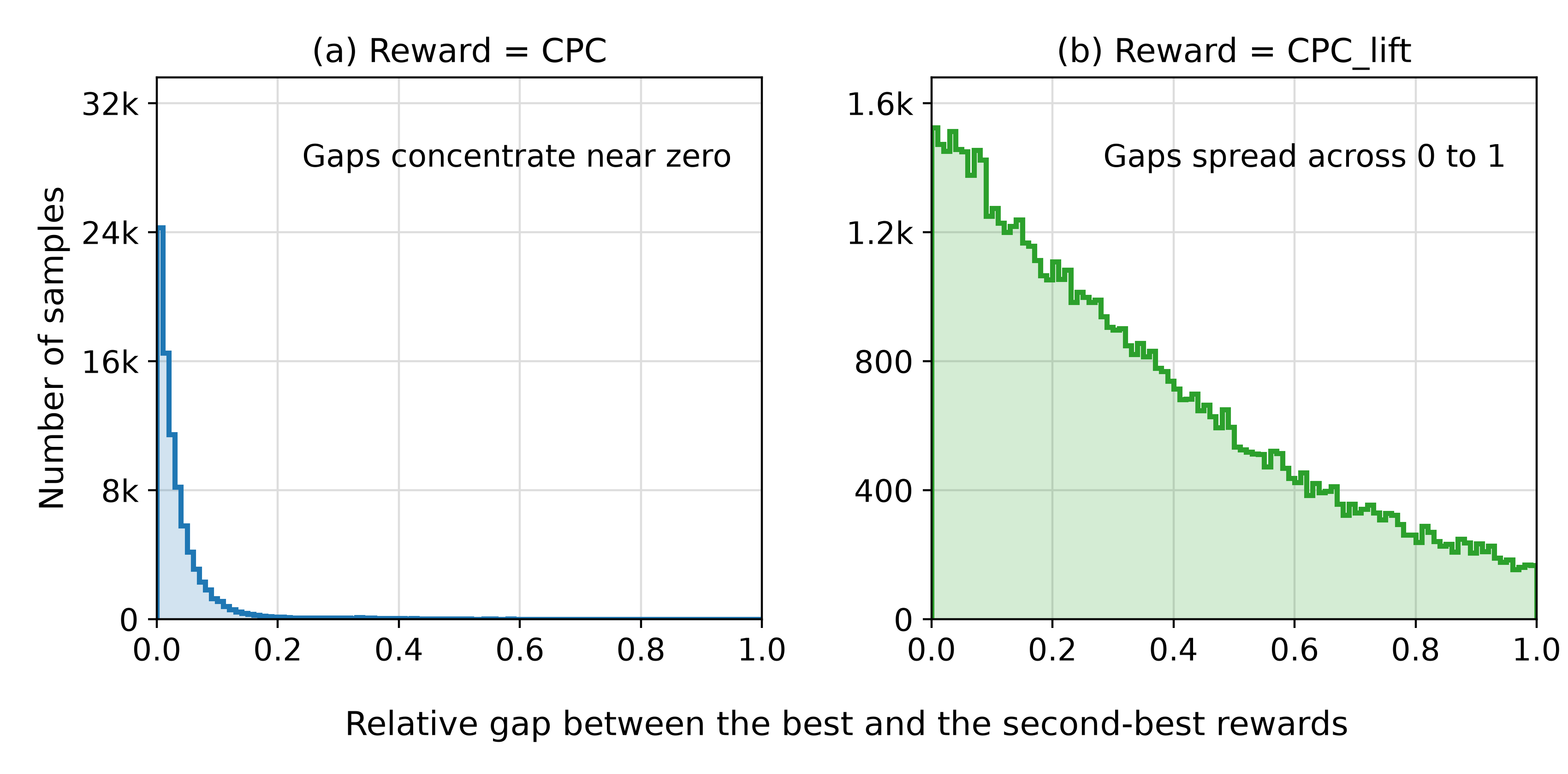
The offline ablation shows this change matters a lot: with raw rewards, revenue lift on a campaign's final day is only 0.08%; with relative lift it is 2.77%, and the CPC reduction on other days widens from 2.17% to 3.02%. These numbers come from offline importance-weighted estimates, so their absolute size cannot be read as online gains, but the direction is clear.
Offline evaluation: how to schedule the cost weight over remaining days
Offline evaluation uses logs from random-exploration traffic: 21 days for training and 7 for evaluation, with inverse propensity scoring (IPS) to estimate a new policy's lift over the production configuration. IPS reweights every log record: during exploration each action is picked at random with probability 1/9, so if the new policy would pick that action with probability 0.5 in the same state, the record's outcome is multiplied by 0.5÷(1/9)=4.5; actions the new policy would never pick get weight 0. Averaging all weighted records estimates "what would have happened under the new policy". Because every action's probability in the exploration logs is known and equal, the estimate has no systematic bias; the price is high variance, which is why the per-day curves below have wide bands.
The authors compare three shapes for how the cost weight changes with remaining days: a step function that switches abruptly on the last day, a linear decline, and an S-shaped curve in between.
| Weight shape | Revenue change | CPC change |
|---|---|---|
| Step | -1.11% | -1.23% |
| Linear (deployed) | +0.05% | -0.34% |
| S-shaped | +1.41% | +0.49% |
Only the linear curve keeps revenue from falling while lowering CPC, so it went to production. Still, its revenue change is only +0.05%, essentially zero; it wins more as "the only option that got worse on neither metric" than as a clear leader on both.
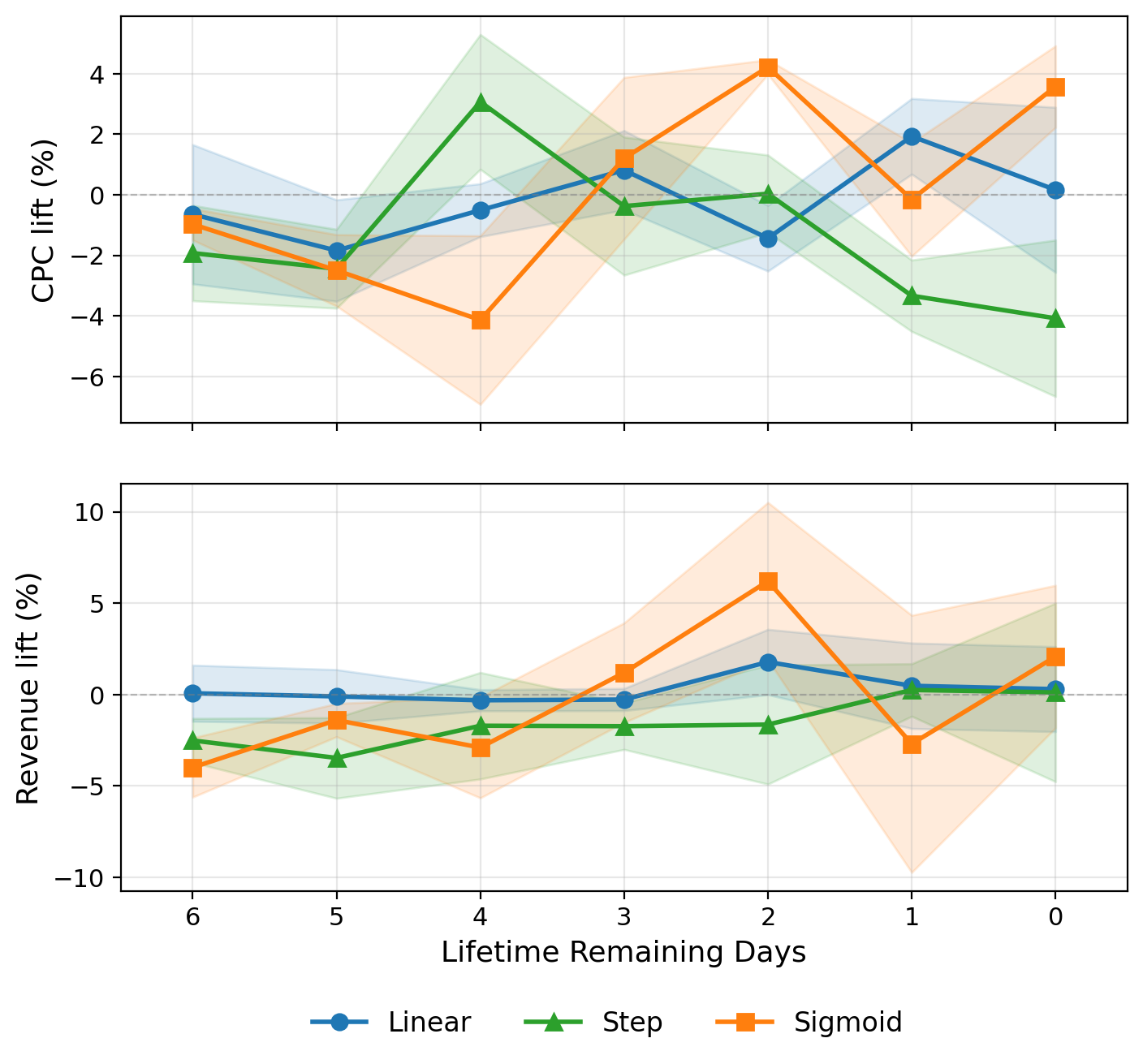
Broken out by day, all three curves have bands that cross 0 on most days, so any single day's number means little; only the aggregated direction is reliable.
Online results
The seven-day online A/B test compares against the default parameters on the same serving infrastructure:
| Metric | All campaigns | Campaigns ending during the test |
|---|---|---|
| Revenue | Flat | +0.43% |
| Clicks | +0.19% | +0.25% |
| eCPC | -0.25% (significant) | +0.18% |
Across all campaigns, eCPC falls a significant 0.25% while revenue stays flat, meaning the same money buys more clicks. For campaigns that ended during the test, revenue and clicks rise while eCPC edges up, which fits the design intent of "prioritize spending near the end".
Split by budget and historical CPC, every segment's eCPC point estimate goes down, most of all for large-budget campaigns (-0.90%, clicks +0.81%) and high-CPC campaigns (-0.64%). That matches intuition: these two groups have the most room for tuning.
Two months after rollout, the authors compared against a small slice of holdout traffic that kept the default parameters. Campaigns more than a week from their end had eCPC almost 1% lower with slightly lower budget utilization; campaigns under a week from the end had slightly higher utilization and still lower eCPC. So the linear weight really does shift the policy from saving to spending late in a campaign. But the holdout traffic is too small, and the authors ran no significance test, so this is only a directional reference.
Limitations as I see them
First, the "reinforcement learning" here is really a contextual bandit. With the discount factor at 0, the model predicts only how today's action affects today's outcome; spending more today leaves less budget for tomorrow, and that cross-day effect is not learned at all, only approximated by the hand-set linear weight. The authors themselves note in the discussion that in a multi-step setting the merged two-head value no longer carries an optimality guarantee.
Second, the gains are small and some numbers are only directional. Across all campaigns eCPC falls 0.25%; for campaigns that ended during the test, eCPC actually rose 0.18%; the two months of post-rollout data have no significance test; in the offline ablation the deployed option's revenue lift is only 0.05%. At this platform's scale a few tenths of a percent has real value, but it should not be read as a clearly large effect.
Third, the exploration cost has to be worked out on your own system. Random exploration needs a slice of each campaign's budget and a separate user bucket, and how large that slice is, how large is, and how many top-K actions to keep all have to be found by trial. Matching the "outcome under the default production configuration", which serves as the reward baseline, to each exploration record also needs its own design. These settings decide how much revenue exploration sacrifices and how high the variance of the offline IPS estimate is. For businesses with few campaigns or small per-campaign budgets, exploration traffic may not be enough to sample all 9 actions well.
How an ads or recommendation team could try it
- First confirm the problem exists: group campaigns by remaining days and budget size, and check whether fixed PID parameters leave systematic gaps in utilization or CPC across groups. If the groups perform about the same, there is little room for tuning.
- Set aside a small independent budget and user bucket for random exploration: three levels each for and , assigned randomly every day, logging "state, action, that day's utilization, that day's CPC".
- Train a two-headed regression model that predicts each action's proportional change relative to the default configuration; evaluate it with IPS on held-out exploration logs before deciding whether to launch.
- Start the merge weight as a simple linear decline, moving from cost first to delivery first as remaining days run out; keep the "one lookup table per day" serving form so the bidder never loads a model.
- Add a fallback: if a campaign's utilization or CPC crosses a threshold, revert it to the default parameters for the day.
Verdict
Letting reinforcement learning pick PID's parameters instead of bidding for it is a very safe compromise between online risk and reward. What is worth borrowing is this deployment form, not the few-tenths-of-a-percent gain.
| Dimension | Assessment |
|---|---|
| Problem importance | High. Fixed budget-control parameters fit poorly across campaign types, a common problem in bidding systems |
| Method novelty | Medium. Parameter-level RL has precedent in control; two-head prediction with merge-at-inference and relative-lift rewards are practical engineering choices |
| Experimental evidence | Medium. A seven-day online A/B test and two months of rollout data, but small gains, untested long-run data, and some undisclosed details |
| Engineering cost | Low to medium. Only one extra lookup table online; the main cost is ongoing random-exploration budget and daily training and inference jobs |
| Worth trying? | Yes, especially for systems that already pace with PID and have very different campaign types; start with small-scale exploration and offline IPS evaluation |
How did this read for you?
Hoot made a note. Thanks for the feedback.

One tap, no sign-in; tap again to undo. Only anonymous counts are kept, never who you are.
Discussion
Add experiment details, reproduction notes or a different take. Requires a GitHub sign-in.
Loading the discussion…