Contents · 6 sections
1How one shop 7 request flows from start to finish2When the model has written only the first token, how does the system know whether shop 7 lies below a branch?3One bit per shop on every branch does not fit in memory4Index memory and the time per check5In the production system, Hit@100 rises from 67.5% to 96.1%6Limits with price ranges, combined conditions and other SID designsSHARE

When generative retrieval must return items from only one shop, filtering after the full item code is generated comes too late. This Shopify paper's fix: every time the model generates one position of the code, the system first checks "if we take this position, does this shop still have anything further down?"
Generative retrieval gives every item a short code called a Semantic ID (SID). The model writes the SID one token at a time from the user's history, and the system then resolves the SID back to items. In Shopify's system an SID has three levels, that is, three tokens, for example 12-305-8 (illustrative, each number is one token). While the model writes tokens, the catalog trie (a prefix tree built from the SIDs that actually exist in the catalog) restricts the next token to continuations that really exist. Beam search then keeps the prefixes with the highest model scores, where a prefix is the part already written, such as 12-305.
The rest of this piece uses one scenario throughout (illustrative): a user in Canada is scrolling the storefront of a small shop (shop 7), and the "you may also like" slot may only show items from shop 7 that can also be sold to Canada.
The difficulty is that the catalog trie only guarantees that a written SID maps to real items. It does not guarantee that those items belong to shop 7, or that they can be sold to Canada. SIDs that start with the same prefix can map to items from several shops. The model's scoring input is only the user history and an optional query, and the condition "shop 7 only" is not part of it, so the items behind the highest-scoring prefixes may well all belong to other shops.
The most direct approach is post-filtering: the system generates as usual, resolves SIDs to items, and then drops items that fail the conditions. The problem is that the beam has limited slots, and the prefixes of items that are later dropped already used up slots during generation. Back to shop 7: suppose the beam width is 2 (only 2 prefixes are kept at each step), and at some step there are four candidate branches, e0 to e3. A branch is a path in the trie that extends the current prefix by one token, which the paper calls an edge. The "items below" a branch are all items whose SIDs pass through that branch. The shops and countries below each branch follow the example in the paper's Figure 3 (shown below), and the model scores are illustrative. With post-filtering the beam looks only at model scores, so it keeps the two highest.
| Candidate branch | Model score (illustrative) | Shops with items below | Any item below sellable to Canada? | Kept by the beam under post-filtering? |
|---|---|---|---|---|
| e1 | 0.40 | Shop 9 | Yes | Kept |
| e3 | 0.30 | Shop 7, Shop 9 | No | Kept |
| e0 | 0.20 | Shop 7, Shop 12 | Yes | Pushed out |
| e2 | 0.10 | Shop 7 | Yes | Pushed out |
Everything below the top-scoring e1 is from shop 9, and nothing below e3 can be sold to Canada, so all items generated from these two branches are dropped at the end. Every item below e2 comes from shop 7, and those that can be sold to Canada were valid results, yet they are never generated because e2 was pushed out at this step. The beam kept only e1 and e3, so in this simplified example the system returns no items at all after filtering.
This paper changes the stage after the model has scored and before the beam selects. RoutingTrie keeps the original catalog trie and adds an index for each item field (attributes such as shop, country, and in-stock status), recording which values occur below each branch. Before each beam selection, the system uses the indexes to exclude branches that lack the required values (for example, no item from shop 7 below), and excluded branches do not enter beam selection. The authors replayed 23,167 historical purchase sessions on the production system, each restricted to the shop of the item the user actually bought. Both approaches use the same model scores. Switching from post-filtering to RoutingTrie raises Hit@100, the fraction of sessions whose purchased item appears among the first 100 eligible items, from 67.5% to 96.1%. Median request latency rises by only 1.1 ms.
How one shop 7 request flows from start to finish
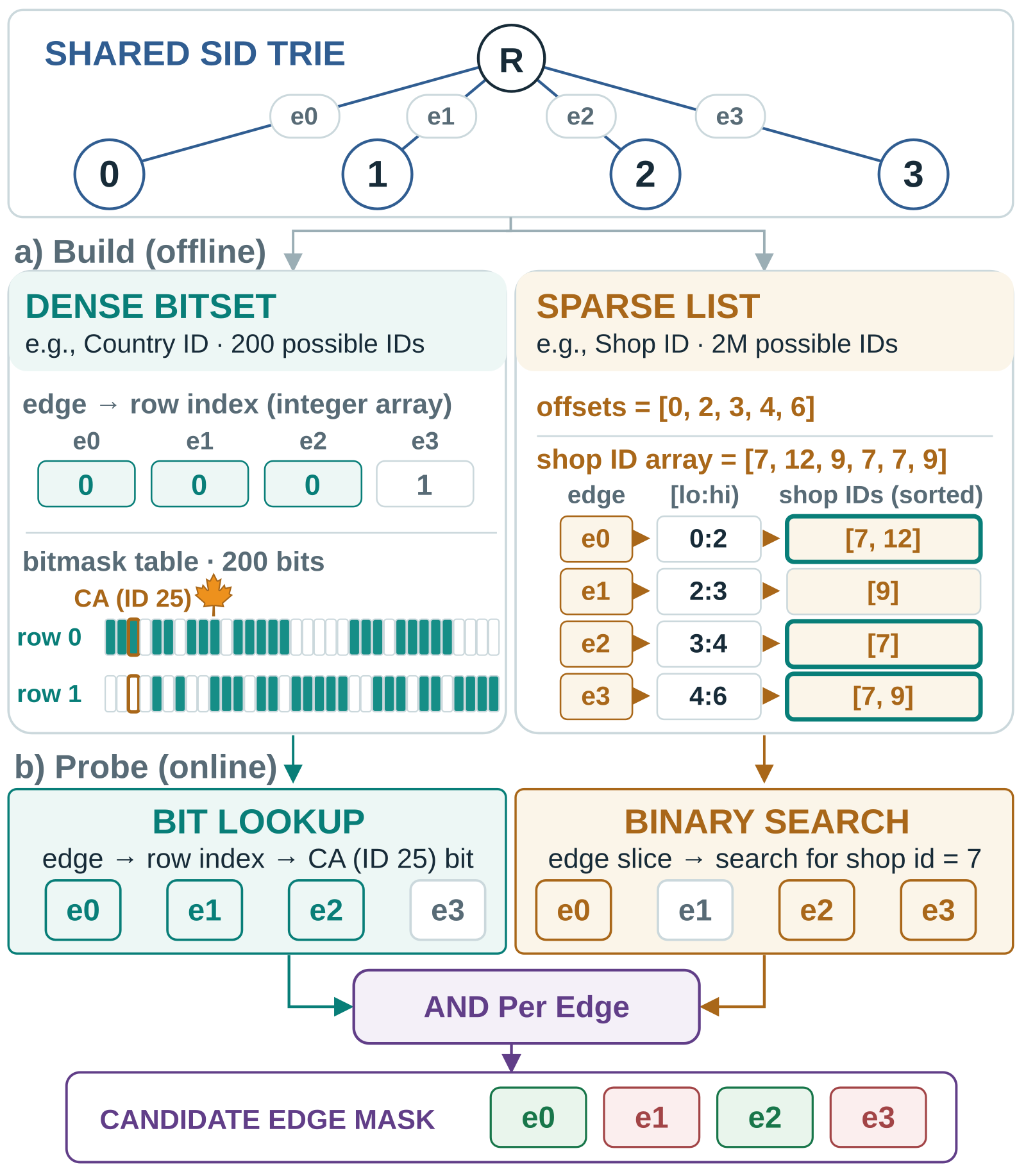
RoutingTrie works in two phases: indexes are built offline, and when a request arrives they are queried each time a token is written. The table below walks through the shop 7 request. The mask in the table is a string of 0s and 1s with one position per candidate branch, where 1 means the branch may enter beam selection.
| Step | Input | Operation | Output | When it runs |
|---|---|---|---|---|
| 1 | All item fields, plus the existing catalog trie | For each field, aggregate upward from the branches at the last SID level, recording the values that occur below each branch | A value set per branch, such as the shop set {7, 12} for e0 | Offline |
| 2 | The value set of each branch | Store each field in one layout (Dense Bitset or Sparse List, described below) | One index per field | Offline |
| 3 | Each prefix in the beam | The trie lists candidate branches and the model scores them | Candidate branches and scores | Each token written |
| 4 | Candidate branches, and the request "country 25 (illustrative, standing for Canada) and shop 7" | Each field queries its own index, and the results are combined by the request's logic (the example here uses only AND; the paper's limitations section says general AND, OR, NOT combinations need extra care when composing branch summaries) | The mask, such as (1, 0, 1, 0), for e0 to e3 in order | Each token written |
| 5 | Model scores and the mask | Pick the top-scoring branches only among those with mask 1 | A new set of prefixes | Each token written |
| 6 | Completed SIDs | Resolve to items and check each item against all request conditions (reason in the next section) | Eligible items | After decoding |
When the model has written only the first token, how does the system know whether shop 7 lies below a branch?
When the model writes the first token, the full SID is still two tokens away, and the system has no concrete item yet. If shops were recorded only at the bottom level, branches in the two levels above could not be judged. So RoutingTrie aggregates upward from the bottom level. The set of a bottom-level branch (the last token of an SID) holds the values of all items sharing that SID. The set of a branch one level up is the union of the sets of the branches below it, because items below those branches all count as being below this branch.
Illustration: SID 12-305-8 covers one item from shop 7 and one from shop 12, and 12-305-9 covers only items from shop 7. Their shop sets are {7, 12} and {7}. Assuming these are the only two SIDs under the prefix 12-305, the set of their parent branch 305 is therefore the union of the two, {7, 12}. This means that when checking 305, the system only has to look up whether 7 is in this set, without walking through the SIDs below one by one.
With these sets, each check is a yes or no answer from each field for each candidate branch. Back to the four branches, treating country ID 25 as Canada (illustrative):
- Shop 7 check: present below e0, e2, e3 and absent below e1; written in order from e0 to e3, the result is (1, 0, 1, 1).
- Country 25 check: present below e0, e1, e2 and absent below e3, giving (1, 1, 1, 0).
- The request requires both conditions, so the two strings are combined position by position with AND (a position is 1 only if both are 1), and the mask is (1, 0, 1, 0), which means only e0 and e2 can enter beam selection.
The mask removes e1 and e3 from selection, and the beam's two slots go to e0 (0.20) and e2 (0.10). The example shows that RoutingTrie leaves the model scores untouched and only changes which branches those scores compete among.
A mask value of 1 on a branch does not mean every item below it is eligible, so step 6 in the table cannot be skipped. One SID can map to several items, and the shop 12 item under 12-305-8 must be dropped once it is resolved.
Because fields are aggregated separately, a branch with no eligible item below it can also pass the check. A mask of 1 on e0 only says that below it there is an item from shop 7 and also an item sellable to Canada, and these may not be the same item. Illustration: the shop 7 item sells only to the US, while the item sellable to Canada belongs to shop 12, so e0 has no eligible item at all. e0 still takes a beam slot, and a lower-scoring branch that does contain eligible items can be pushed out. The authors therefore state explicitly that with a finite beam, RoutingTrie cannot guarantee that no eligible item is lost. For requests where several conditions must all hold, what the mask can exclude with certainty is only branches that lack a required value entirely.
One bit per shop on every branch does not fit in memory
The check logic is simple; the hard part is storing these sets. ShopTrie, a test catalog the authors generate themselves, has 338 million branches, and every field must store a set on every branch. The fields also differ widely: in-stock status has only 2 values, country has 240, and shop has about 1.9 million. In real catalogs, for fields with only two values, the values present below a branch average more than 50% of all possible values, while for category and shop this ratio is below 0.1%. A single layout can hardly suit both fields with few values and full sets and fields with many values and sparse sets, so the authors provide two.
Fields like country use Dense Bitset: each country gets one bit, each branch corresponds to a row of 0s and 1s, and a query checks whether the relevant bit is 1. Many branches have exactly the same set of countries below them, so each distinct row is stored once and each branch only records which row it uses.
Illustration: there are 1,000 branches, each row takes 8 bytes, and there are only 2 distinct rows. Storing one row per branch takes 8,000 bytes. With shared rows, the 2 rows take 16 bytes and the 1,000 four-byte row numbers take 4,000 bytes, for 4,016 bytes in total, a saving of almost half. In the paper's Figure 3, e0, e1, e2 share one row and e3 uses another, and the earlier (1, 1, 1, 0) is obtained exactly this way: the system reads the row number once, then reads bit 25 of that row. Two array reads suffice, and the number of countries does not change the step count.
Applying the same approach to the shop field breaks down. With about 1.9 million shops, a row must reserve about 1.9 million bits even when only one shop lies below the branch. In fact a branch has only 2.71 shops below it on average, with a median of 1, so nearly all bits are empty. The authors estimate that a Dense Bitset for the shop field would take 22.4 TiB.
Sparse List stores only the shops that actually occur. It sorts each branch's shop IDs, concatenates them all into one large array called values, and uses an array called offsets to record where each branch starts and ends, the same layout as CSR (compressed sparse row, a format that stores only nonzero entries and where each row starts and ends) for sparse matrices.
The illustration uses the data from the paper's Figure 3 directly: values is [7, 12, 9, 7, 7, 9] and offsets is [0, 2, 3, 4, 6]. To check whether e1 has shop 7, entries 1 and 2 of offsets (counting from 0) are 2 and 3, so e1's shops occupy values from index 2 up to but not including index 3, which is [9]. Binary search does not find 7, so the result is 0. For e0 the range is [7, 12], 7 is found, and the result is 1. The number of comparisons in binary search depends only on how many shops lie below the branch, not on how many shops exist across the catalog. Storing the shop field as a Sparse List measures only 5.92 GiB, and the Dense Bitset estimate is about 3,900 times that.
Which layout is smaller depends on how many values a field has and how much the branch sets repeat. The authors compare the bytes each layout uses and derive a selection rule: Dense Bitset uses less memory when
Here I is the average number of values below a branch, M is the total number of possible values in the field, E is the number of branches, and D is the number of distinct rows in Dense Bitset. Dense Bitset takes bytes (each branch's row number plus the distinct rows). Sparse List takes bytes (all stored IDs plus offsets). Comparing the two gives the rule above. A smaller D/E means more repeated rows. Intuitively, a larger M makes each row longer and Dense Bitset more expensive; a larger I means more IDs to store and makes Sparse List more expensive; more repeated rows make Dense Bitset cheaper. When E is large, the final 2/E term is small enough to ignore.
The paper gives an example you can do in your head: with M = 16,384, M/64 equals 256. At D/E of 0.10 the threshold (the right-hand side of the rule; Dense Bitset is smaller when I exceeds it) is 2×0.10×256−1, which comes to about 50; when D/E drops to 0.01 the threshold is about 4. So for the same field, more repeated rows relax the condition under which Dense Bitset pays off from an average of 50 values to 4.
Plugging in the paper's fields makes the choice clear. For country, M is 240 and M/64 rounded up is 4; the number of distinct rows cannot exceed the number of branches, so D/E is at most 1 and the threshold is at most about 7, while the actual I is 62.95, so the rule picks Dense Bitset. For shop, M/64 is about 30,000; taking D/E as 0.01 for illustration gives a threshold of about 600, while the actual I is only 2.71, so the rule points to Sparse List. The rule assumes 32-bit IDs and 64-bit bitset words, and the authors' actual implementation redoes the comparison with the real widths of the stored arrays, using the same logic.
Index memory and the time per check
Once the layouts are chosen, the question is how much memory the indexes actually use and how long one check takes. ShopTrie always generates the same trie and item fields from the same configuration and random seed, and some field distributions are calibrated to statistics from real catalogs, so different methods can be compared on identical inputs. This experiment uses three SID levels, 8,192 tokens per level, 8 fields, and beam width 64. Latencies in the table are summed over the three SID levels and cover only field checks and mask generation, excluding model scoring and beam selection.
| Component | Number of values | Average values per branch | Layout | Memory (GiB) | CPU total over three levels (ms) | GPU total over three levels (ms) |
|---|---|---|---|---|---|---|
| In stock | 2 | 1.24 | Dense Bitset | 0.31 | 0.10 | 0.08 |
| Country | 240 | 62.95 | Dense Bitset | 1.33 | 0.26 | 0.08 |
| Category | about 5.6K | 1.38 | Sparse List | 1.01 | 0.67 | 0.08 |
| Shop | about 1.9M | 2.71 | Sparse List | 5.92 | 1.26 | 0.09 |
| Shared trie (338 million branches) | - | - | CSR (the trie's connectivity is stored in this format too) | 0.77 | - | - |
| Total (including the 4 fields not listed: on sale, condition, sales channel, fulfillment) | - | - | - | 10.91 | - | - |
The trie plus the indexes for all 8 fields take 10.91 GiB, and the shop field alone accounts for more than half. This shows that memory goes mainly to fields with very many values, like shop.
Across the 8 fields, the number of values ranges from 2 to about 1.9 million, yet the mean GPU total for the three levels stays between 0.075 and 0.087 ms. This shows that on GPU, the number of values in a field barely affects the cost of checking. The reason is that Dense Bitset tests a single bit and Sparse List binary-searches only a very short segment: category and shop have only 1.38 and 2.71 values per branch on average, so the search finishes quickly.
On CPU, latency differs by more than ten times across fields, from 0.10 ms for in-stock to 1.26 ms for shop. When beam width grows from 8 to 256, CPU check latency for the shop field rises from 0.43 ms to 2.67 ms, while GPU latency rises only about 7%. This shows that field checks get more expensive with the beam on CPU, while on GPU beam width puts almost no pressure on them.
The cost of picking the wrong layout falls mainly on memory. When the authors switch in-stock and country to Sparse List, memory becomes about 9 and 17 times that of Dense Bitset; switching category to Dense Bitset makes it about 10 times the size of Sparse List. Across these same swaps, GPU latency differs by only 2% to 6%. This shows that on GPU, choosing the memory-saving layout by the rule does not cost speed. On CPU, category would be about 2.4 times faster as a Dense Bitset, at the price of that 10 times memory.
When an item sells out, the value of the in-stock field changes and the index must follow, but the SID trie stays unchanged. The system recomputes only the sets of affected branches (the bottom-level branch holding the item and the branches above it), then refreshes the corresponding field index on the GPU. Updating 0.01% of bottom-level sets (about 32,000 branches) takes 0.077 to 0.093 seconds for each of the 5 small fields such as in-stock, 6.288 seconds for category, and 19.530 seconds for shop. Shop is slow because values is one contiguous array: when a branch's set grows or shrinks, the current Sparse List implementation must repack the array, while a short bitset only flips the relevant bits and can be patched in place. This shows that fields like in-stock status can be refreshed within 0.1 seconds, while refreshing the shop field takes more than two hundred times as long.
In the production system, Hit@100 rises from 67.5% to 96.1%
The synthetic ShopTrie catalog can only measure memory and latency; item recovery has to be measured on a real system. The authors replayed 23,167 historical purchase sessions on their production system, whose model has 14 billion parameters, with a three-level trie of 8,192 tokens per level and beam width 100. Each session uses the item the user actually bought as the target and that item's shop as the filter condition. Each session is thus a "items from one shop only" request, with the shop set to the one the user actually ordered from.
Post-filtering and RoutingTrie use the same model scores, and the only difference is whether filtering happens before beam selection or after generation ends. Hit@100 rises from 67.5% with post-filtering to 96.1% with RoutingTrie, a gain of 28.6 percentage points. Since the only difference is when filtering happens, this shows that recovering these extra purchases does not require a new model; they were previously pushed out during beam selection.
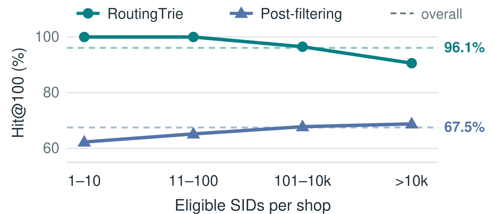
Grouped by shop size, the largest gap between post-filtering and RoutingTrie appears precisely for small shops like shop 7. For shops with only 1 to 10 eligible SIDs, Hit@100 rises from 62.3% to 100.0%, and the other groups gain 21.8 to 34.8 percentage points.
My reading is this: under a single-shop condition, a prefix that passes the mask has at least one SID of that shop below it. A small shop has at most 10 eligible SIDs, so at most 10 prefixes pass the mask at each level, which fits easily in 100 beam slots, and none of those SIDs is pushed out. Keeping all the SIDs is only a precondition, since the purchased item must also rank among the first 100 eligible items after SID resolution; the measured Hit@100 for this group is 100%, so nothing was lost at that stage in these sessions either. Under post-filtering, these few prefixes compete with prefixes from the whole catalog for the same 100 slots. For larger shops, more than 100 prefixes may pass the mask, so the beam still has to choose by model score and the purchased item can still be pushed out, which is why overall Hit@100 stops at 96.1%. Hoot says

- Illustrative: the target shop has only 2 SIDs, so the beam truncates nothing. A holds 60 eligible items and B holds 70, with the target item in B, for 60+70=130 items, 30 more than 100.
- If A were expanded first, B would have only 100−60=40 positions left, and 30 of its items would miss the top 100. Whether the target item hits depends on expansion and ordering.
The item counts are illustrative. The paper defines Hit@100 over the first 100 eligible items after SID resolution, and does not say how items sharing a SID are expanded or ordered, so we cannot claim that ordering affects item-level hits only once prefixes exceed the beam. The 100% for this group is a replay measurement; beam capacity explains only why the SID is not truncated.
Source
paper §5.2 Hit@100 definition (first 100 eligible items after SID resolution) and results by shop size; §4.1 one SID may represent multiple items with different metadata; the item counts of SIDs A and B are illustrativeLatency was measured on an H200 over the full GR (generative retrieval) pipeline, including model inference, SID decoding, field checks, and beam selection. With RoutingTrie storing the shop field as a Sparse List, median request latency goes from 27.1 ms to 28.2 ms. This shows that in this system, moving filtering into every step costs only 1.1 ms more.
These numbers answer whether the purchased item can be recovered when a request is already restricted to a single shop. The filter condition is taken directly from the purchased item, so this Hit@100 measures recovery rate, not conversion or revenue.
Limits with price ranges, combined conditions and other SID designs
RoutingTrie's indexes work only with discrete values, so numeric fields such as price must be bucketed first. Illustration: one bucket covers 50 to 100 dollars and the request wants items under 80 dollars; the index records only buckets, so a branch whose items are all priced at 90 dollars still passes the check, and resolved items must be checked against the original condition again.
A combined condition such as shop 7 plus Canada falls outside the production replay. The replay used only a single shop condition, so this Hit@100 cannot tell how much loss comes from cases like e0, where both conditions pass separately but no single item satisfies both.
The paper's memory, latency, and Hit@100 results all rest on a design with residual codebooks plus a catalog trie. With other SID constructions such as independent codebooks, as long as a trie is still used, the approach of checking which values lie below a branch before beam selection still applies, but the memory and latency numbers above do not carry over directly.
Back to the user browsing shop 7: the model's scores did not change at all; what changed is that the beam's two slots moved from e1 and e3 to e0 and e2. RoutingTrie adds only two things to the system: one index per field recording which values lie below each branch, and a check before every beam selection.
How did this read for you?
Hoot made a note. Thanks for the feedback.

One tap, no sign-in; tap again to undo. Only anonymous counts are kept, never who you are.
Related papersMore from Paper Daily
 Generative · 2026-08-07Recall Is Not Enough: A Reader-Context Diagnostic for Budget-Constrained Retrieval-Augmented GenerationDeep dive: Recall Is Not Enough: A Reader-Context Diagnostic for Budget-Constrained Retrieval-Augmented Generation.
 Generative · 2026-11-05ZeroGR: Filtering-First Constrained Decoding for Generative RecommendationEngineering teams serving generative recommenders should read this: it shows that most constrained-decoding compute goes to candidates that will be discarded, and gives a filter-first system implementation. Generative recommenders emit item codes one token at a time, and every step must keep the code pointing at an item that really exists in the catalog. The usual approach scores every possible n…
 Generative · 2026-11-02RoFiGR: Coarse Routing, Fine Refinement via Level-Adaptive Distillation in Multimodal Generative RecommendationA generative recommender produces an item's SID one code at a time, and once the first two codes pick the wrong branch, no amount of later precision can recover the relevant items. In multimodal recommendation the SIDs are mostly built from image and text semantics, so their first codes may not reflect which items the same users tend to buy. RoFiGR therefore concentrates collaborative signal on t…
Discussion
Add experiment details, reproduction notes or a different take. Requires a GitHub sign-in.
Loading the discussion…