Contents · 5 sections
1Freeze the recommender and add a two-direction correction to its score2Learn the correction on the previous day, then only calibrate it today3Give each user a mix of 8 coefficient sets, so one video is corrected differently for different users4Most of the gain comes from pretraining on the previous day5Small gains, a loss to category groups on MF, and about 10× slower inferenceSHARE

SAGE-PAIR shows that when a new day brings labels for only one exposure in two hundred, you are better off not learning new parameters with them, and instead only calibrating a score correction that was already learned the day before and has just two item-side directions.
Recommender systems are usually updated on a daily rolling schedule. When a new day starts, the deployed model keeps ranking videos, but whether a user clicked only becomes known once outcomes flow back. By the next ranking update, only a small fraction of the day's exposures have outcomes. The paper studies budgets from 0.05% to 1%, and the main experiment uses 0.5%.
Take May 28 from the paper's experiments. That morning the system has a recommender trained on data from the previous few days. The day's exposure pool holds over a million exposures, but only about 5.8K have click outcomes before the update, so the signal available for updating is one exposure in two hundred. The rest of this piece follows that day.
The difficulty is that this day already looks different from the day before. Only 29.0% of the videos seen on May 28 also appeared on May 27, and only 48.8% of users overlap. A recommender not trained on either day sees its Macro-AUC fall from 0.553135 on May 27 to 0.546759 on May 28. So the model does need to change, but 5.8K outcomes are far fewer than a recommender's degrees of freedom, and they cannot tell you which way to change it.
The most direct option is to fine-tune the whole recommender on those 5.8K outcomes. User, item, and interaction parameters all move, and the authors argue that each parameter receives very little useful signal. The paper ran this control on KuaiSAR-small: after full-model fine-tuning, NDCG@10 went from 0.626024 to 0.626048, so it brought almost no gain. Switching to LoRA or an Adapter that trains only a few hundred parameters does not remove the problem. Those modules learn a transformation of the recommender's internal representations, several layers away from "which videos should move up today", and 5.8K outcomes still struggle to pin it down.
Freeze the recommender and add a two-direction correction to its score
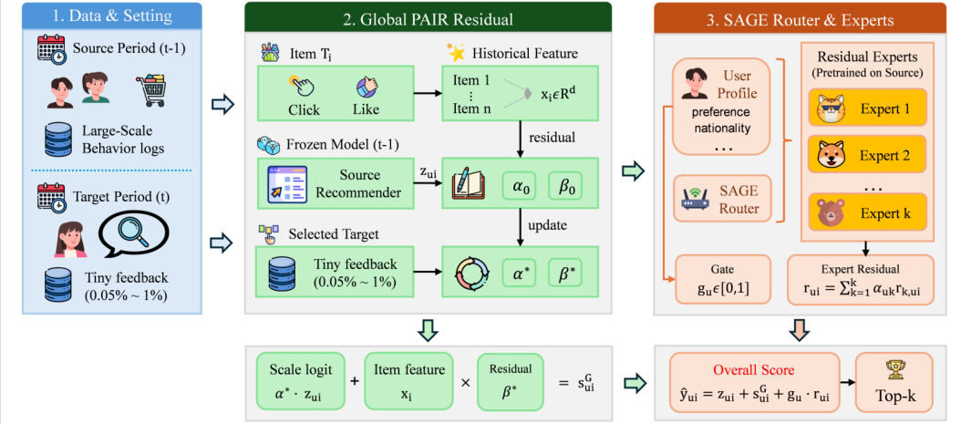
SAGE-PAIR starts from a simple idea: if labels are scarce, restrict what they can change to a very small number of directions. The recommender is fully frozen and gives each user–video pair a raw score . The correction only adds or subtracts a little from that score.
The paper calls the basic global correction PAIR (a small residual added to the frozen score, shared by all users). Its score is:
Here holds the video's click rate and like rate from the previous window, and are their weights, and rescales the raw score. The item side is just these two numbers, not a learned embedding. The authors' intent is to stop scarce labels from identifying a free item representation. The labels only decide whether a video with a high click rate yesterday should move up a bit today, and likewise for like rate.
Both statistics are shrunk first. Illustration: a video was shown only 4 times yesterday and liked twice, so its raw like rate is 0.5. With a site-wide like rate of 0.05 and the paper's α=20, the shrunk rate is (2+20×0.05)/(4+20)=0.125. Videos with few exposures are pulled back toward the site average, so a few lucky likes cannot become a large correction direction. The shrunk values are then standardized by the site-wide mean and standard deviation, so the penalties on the two behaviors are on the same scale.
What about videos that did not appear the day before? About seven in ten videos on May 28 fall into this case. Working through the formula, their exposure and click counts are both 0, so the shrunk rate equals the site-wide average. After standardization every new video gets the same constant two-dimensional feature, and the correction gives all of them the same boost.
The scale carries an penalty. Without it, the model could fit the 5.8K outcomes by stretching or shrinking all raw scores, which amounts to passing off rescaling as retraining. The penalty keeps to a small calibration.
Illustration: video V was clicked a lot yesterday but rarely liked, so after standardization . If the learned , its correction is 0.3−0.1=+0.2, the same for every user.
Learn the correction on the previous day, then only calibrate it today
A global correction with only three parameters still wobbles when fitted on 5.8K outcomes. So the second step of SAGE-PAIR is to train the same correction first on the previous day's complete labels. All outcomes from the previous day have arrived, giving 1.23M rows; today's few outcomes only continue the optimization from there.
Both stages use the same objective. Each labeled (user, video, clicked or not) row gets its own binary cross-entropy, plus an L2 penalty that pulls toward 0 and toward 1, keeping the score close to the frozen model's raw score. This is a pointwise click-prediction loss, not a pairwise ranking loss.
| Step | Data | What happens | Output |
|---|---|---|---|
| 1 | May 22–26 | Train the recommender, then freeze it | Raw score |
| 2 | Source data before May 28 | Compute each video's click and like rates and each user's profile | Fixed and user profiles |
| 3 | May 27, 1.23M rows | Keep the recommender fixed, train the correction for 5 epochs | Initial correction state |
| 4 | May 28, 0.5% (about 5.8K rows) | Continue training from step 3 for 8 epochs | Final correction |
| 5 | May 29–31 | Score, rank, evaluate | NDCG@10 and others |
Step 3 supplies a starting point, not a constraint. In step 4 every parameter is copied from the previous day's state and then updated only on May 28 outcomes. The paper calls the version that uses only the new day's labels target-only PAIR, and the version pretrained on the previous day source-pretrained PAIR. Hoot says

① Previous-day pretraining (May 27)
- Training data
- All of that day's returned outcomes, 1.23M rows
- Parameters updated
- All of them: the scale, the two global weights, the routing matrix, the 8 expert sets
- Epochs
- 5 epochs
- Correction for video V (illustrative)
- x=(+1.0, −0.5), β=(0.3, 0.2), correction 0.3−0.1=+0.2
② New-day calibration (May 28)
- Training data
- An outcome-blind uniform 0.5% of the day's exposure pool, clicks revealed only after the rows are fixed, about 5.8K rows; not whichever outcomes arrive first
- Parameters updated
- Still all of them, copied from ①'s state and trained further; no direction is locked
- Epochs
- 8 epochs, on these 0.5% rows only
- Correction for video V (illustrative)
- x unchanged, β calibrated to (0.1, 0.4), correction 0.1−0.2=−0.1
Neither stage touches the recommender, each video's two-dimensional feature x (click rate, like rate) or each user's profile. They are computed before the new day's labels arrive, so the correction can only ever add or subtract along these two features; the previous day only decides which weights learning starts from.
The two columns are the two training stages of the same correction; the footer lists what neither stage touches. Video V's coefficients are illustrative, showing that calibration on the new day can flip the same video's correction from a boost to a penalty.
Source
paper §4.1 (item features and user profiles come from source-period interactions and are then fixed); §3.3, §4.2 (x and profiles fixed before target labels are accessed; only the correction parameters update); §4.3, §4.5 (5 epochs of previous-day pretraining; in the target stage every parameter is copied from the source state and trained 8 more epochs, "an initialization, not a constraint"); §3.2, §5.1 (outcome-blind uniform sample of the exposure pool, labels revealed only after the rows are fixed, 0.5%, about 5.8K rows); Table 1 (1.23M May 27 rows)My reading is that this step lets 1.23M rows decide which direction to correct, and leaves how much to correct for 5.8K rows to tune. The previous day and today share the same system and the same video features, so directions learned yesterday mostly still apply today.
Give each user a mix of 8 coefficient sets, so one video is corrected differently for different users
The global correction is the same for every user. Yet a video that is clicked a lot but rarely liked may deserve to move up for users who love gaming and down for users who love food. Learning a separate correction for each kind of user from 5.8K outcomes alone lands exactly where labels are least sufficient.
SAGE-PAIR (Core) prepares 8 coefficient sets (the paper calls them experts). Each set has just two numbers, one for click rate and one for like rate. Every user has a fixed profile: a click histogram over 37 first-level categories plus two activity slots, 39 dimensions in total. A small routing matrix turns the profile into weights over the 8 sets, and the weights sum to 1. The user's personal coefficients are the weighted sum of the 8 sets.
Users who did not appear the day before have no profile. The paper spells out a fallback: such users drop the expert term and use source-pretrained PAIR, and when there is no adjacent previous day at all, the system falls back to target-only PAIR.
Illustration, assuming only two sets matter: set 3 is (0.2, 0) and set 5 is (0, 0.4).
| User | Weight on set 3 | Weight on set 5 | Personal coefficients | Extra correction for video V |
|---|---|---|---|---|
| Gaming fan | 0.8 | 0.2 | (0.16, 0.08) | 0.16−0.04=+0.12 |
| Food fan | 0.2 | 0.8 | (0.04, 0.32) | 0.04−0.16=−0.12 |
Video V first gets the global +0.2, then +0.12 or −0.12 depending on the user. This table is what the correction finally produces in serving: one pair of coefficients per user.
The routing matrix and these sets are also pretrained on the previous day and calibrated on the new day. Counting the global weights and the scale, the whole Core version has 331 parameters.
Because each set has only two numbers, the sets span at most two directions. They are not independent predictors, only anchors in the same two-dimensional space. Each user interpolates between the anchors by weight, so the correction always stays on the click-rate and like-rate directions.
The paper also has a SAGE-PAIR (Full) version that adds a 0-to-1 gate computed from the profile (multiplied onto the expert correction) and a search-behavior profile. The ablations later show that both additions matter little.
Most of the gain comes from pretraining on the previous day
The paper reports results by cell. A cell is one combination of a recommender seed and a sampling seed; within a cell both methods use the same recommender and the same labeled sample, and differences are taken cell by cell. In the locked KuaiSAR-v2 experiment (5 recommender seeds × 5 sampling seeds, 25 cells), SAGE-PAIR (Full) raises NDCG@10 from 0.615217 for target-only PAIR to 0.626115, a 1.77% relative gain, positive in all 25 cells. Recall@10, NDCG@20, Recall@20 and Macro-AUC all move up too. This shows the gain is not an accident of one cutoff.
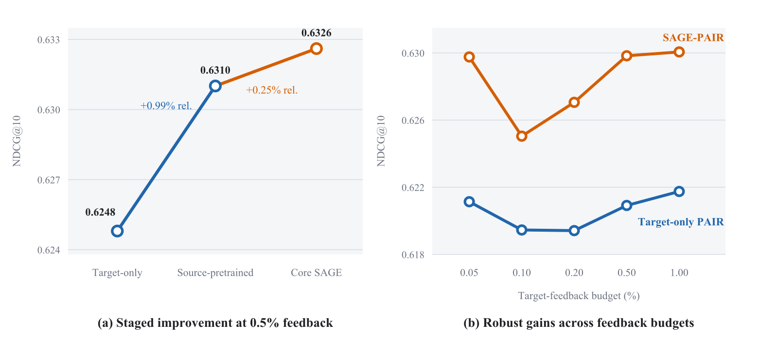
The more important step is splitting that gain apart. In a separate fair comparison (3 recommender seeds × 5 sampling seeds, 15 cells), target-only PAIR scores 0.624800, source-pretrained PAIR rises to 0.631008 (+0.99%), and SAGE-PAIR (Core) reaches 0.632608 (a further +0.25%). This shows both steps help, but by very different amounts.
The target-only PAIR reference differs across experiment batches, so numbers from different batches cannot be compared directly.
With the same 0.5% of labels, most of the gain comes from pretraining on the previous day (+0.99%), and the per-user experts add only another quarter of a percentage point.
A natural question: if LoRA and Adapter are also pretrained on the previous day, do they work as well? The paper ran this comparison. LoRA and Adapter are both rank 4 with 256 trainable parameters each, close to the Core version's 331. FOMAML-LoRA is a meta-learning approach: it cuts many small tasks out of the earlier five days, learns a LoRA initialization that is easy to fine-tune quickly, and then updates on the May 28 labels.
| Method (same batch of 15 cells, 0.5% labels) | NDCG@10 change vs. frozen model | Positive cells |
|---|---|---|
| target-only LoRA | +0.000172 | 11/15 |
| target-only Adapter | +0.000462 | 12/15 |
| FOMAML-LoRA | +0.000189 | 12/15 |
| LoRA pretrained on previous day | −0.000372 | 3/15 |
| Adapter pretrained on previous day | −0.000553 | 4/15 |
| source-pretrained PAIR | +0.028814 | 15/15 |
| SAGE-PAIR (Core) | +0.030407 | 15/15 |
This shows that pretraining on the previous day is not a cure-all by itself. At a similar parameter count, LoRA and Adapter get slightly worse after pretraining, while the PAIR correction is positive in all 15 cells and much larger. The authors' explanation is that LoRA and Adapter learn a transformation of the recommender's internal representations, several layers away from today's ranking, while PAIR learns its correction directly on two observable directions, click rate and like rate. The paper supports this explanation with controlled comparisons, but it does not measure directly whether the update directions are identifiable.
In the ablations, replacing the learned router with fixed k-means groups reaches only 0.621232 NDCG@10, against 0.628131 for the learned soft router (reference 0.619675). Removing the gate gives 0.628203 and removing the search profile gives 0.627694, almost no difference. With 4, 8 or 16 experts the scores are 0.627674, 0.627783 and 0.627890, also flat. This means the parts that matter in the Core version are previous-day pretraining and the learned router, and the gate and search profile can be dropped.
Over 12 consecutive rolling days, continuing each day from the previous day's correction gives an average NDCG@10 of 0.645916. That is slightly better than restarting each day from the May 27 state (0.645407) and higher than a PAIR re-estimated on all sampled labels so far (0.640139). This shows the correction can be carried forward day after day.
Small gains, a loss to category groups on MF, and about 10× slower inference
First, the absolute gain is small. In the locked experiment the absolute NDCG@10 increase is about +0.0109, and user routing adds only 0.25% in the fair comparison. If what matters to you is personalized correction, the evidence here mainly supports the global correction plus previous-day pretraining.
Second, there is an exception when the recommender changes. On Two-Tower, SAGE-PAIR (0.624925) beats the strongest user-preference group baseline (0.622833) by 0.34%. But on MF, SAGE-PAIR scores 0.637496, below a simple baseline that groups by item category at 0.638137.
Third, the label-budget curve is not monotone. Across five budgets from 0.05% to 1%, SAGE-PAIR beats target-only PAIR every time, but the 0.10% budget has the smallest relative gain (0.90%) and is positive in only 22/25 cells. The authors explain that in a fixed exposure pool, the label count alone does not determine how many contrasts of the same user both clicking and not clicking are observed. This pairable fraction is a diagnostic the authors use after the fact to interpret the budget curve; it does not enter the loss or training. It means more labels do not necessarily buy proportionally more gain.
Fourth, training is cheap and inference is not. Staged training takes only 0.606 seconds, against 22.166 seconds to retrain the recommender.
Inference is a different story. On an RTX 4090 the paper runs end-to-end inference over all 2,255,520 rows in one pass and reports the median time: 18.472 ms for the frozen model and 183.201 ms with SAGE-PAIR, about 10 times as long. This is the time for the whole batch, not per-request latency. The paper calls it compatible with millisecond-scale serving; this means a team planning to deploy it should first measure this overhead in its own serving path.
Back to the 5.8K outcomes from May 28: SAGE-PAIR does not ask them to learn a new model, only to fine-tune 331 numbers already trained the day before. The paper's strongest conclusion is that this step of pretraining on the previous day brings most of the gain; the 8 per-user coefficient sets add only a small further step on top.
How did this read for you?
Hoot made a note. Thanks for the feedback.

One tap, no sign-in; tap again to undo. Only anonymous counts are kept, never who you are.
Discussion
Add experiment details, reproduction notes or a different take. Requires a GitHub sign-in.
Loading the discussion…