Contents · 8 sections
1Where a 2 KB state comes from2One action can write into several channels at once3Each channel decides how long it remembers4Finally each fusion vector becomes one 64-bit integer5Update after every action, export only at requested timestamps6The last 64 actions take 262,144 bytes and are still 3.98% below 2 KB SeqFold7Ablation differences for channel count, fusion layers, and decay type8The same codes go to search and QACSHARE

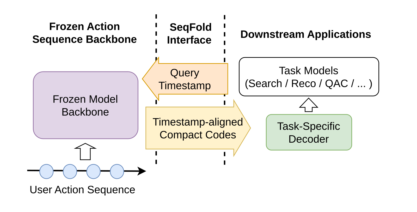
Coupang's SeqFold is about handing a frozen long-history user sequence model to downstream teams: each downstream record only needs "the user state before that moment", so exporting one 2 KB code at the requested timestamp is enough.
Coupang has a trained, periodically refreshed user action sequence model: a 4-layer Transformer with hidden size 256, reading up to 2,000 actions per user, about 1,700 on average. Its main task is predicting which type the user's next action will be. Search, recommendation, and QAC (query autocomplete, which completes a half-typed query) all want to reuse what it knows about the user, without retraining it or changing its architecture.
The hard part is the shape of a downstream record. Take one illustrative example through the whole piece: a user with 1,700 actions runs a search at 9 p.m. on Tuesday. When the search model uses that search as a training record, it may only use actions before 9 p.m.; otherwise it peeks at the answer. Passing the raw backbone output as is means 1,700 actions × 4 layers × 256 dimensions, or 1,740,800 floats, about 6.96 MB in FP32. A downstream record normally has only a few hundred features.
The authors compare several baselines that keep only part of the information, including truncation, pooling, and sampling. The most direct is truncation: store only the hidden states of the last 64 actions. In the illustrative example, the user browsed strollers repeatedly three months ago, and the last 64 actions are all comparing phone cases, so after truncation the search model no longer sees the strollers. Another is averaging all last-layer actions into one 256-dimensional vector, which blends strollers and phone cases until neither can be told apart. Yet another is a static per-user embedding, but it is aligned to the moment it was computed; a training record from last month that uses an embedding computed today mixes in actions that happened after the record.
SeqFold adds a compression interface after the backbone. A downstream system queries it with a timestamp, and it returns the state before that time, at a fixed size of 2,048 bytes. On the authors' proprietary data this is about 3,400 times smaller than storing the full multi-layer hidden states, while the upstream metric is only 2.11% lower (relative) than the full states.
Where a 2 KB state comes from
Start with the full path for one user and one timestamp. The backbone stays frozen; SeqFold only reads the hidden state it computes for each action at each layer. The backbone is causal, and each historical action's hidden state only sees the actions before it, so taking only the states before the target time never sees the answer.
| Step | Input | Operation | Output | Training only |
|---|---|---|---|---|
| 1 | The user's action sequence | Frozen backbone encodes it layer by layer | One 256-dim hidden state per action per layer | No |
| 2 | Each action's hidden state at one layer | 64 independent gates each give a weight between 0 and 1 | How much of this action goes into each channel | No |
| 3 | Weighted actions | Accumulate with each channel's own time decay | 64 continuous 256-dim vectors per layer (fusion vectors) | No |
| 4 | Fusion vectors | RMSNorm, then LFQ quantization | 64 64-bit integers per layer | No |
| 5 | Codes | A training decoder restores them, the current action cross-attends to them, scored with the backbone's own action-prediction objective | Gradients for training the compressor | Yes |
| 6 | Codes | Each downstream learns its own decoder with a chosen output size, then cross-attends | User features for the downstream model | No |
A "channel" here is one of the 64 accumulators SeqFold keeps per layer, each holding one 256-dim vector. Step 5 exists only to train the compressor and is dropped afterwards; what downstream receives is the code from step 4. The next sections take steps 2 to 4 apart. Hoot says

- Illustrative: to predict action 4, the code Q₃ holds only actions 1–3, which is i = 3 and i+1 = 4 in the paper's Eq. (4).
- The query uses action 4's context view. The paper splits each action into a context part and a label part; with the full view instead, the label would already be in the input, like answering with the answer key open.
- Each layer has 64 codes of 64 bits each; how a 256-dim fusion vector becomes 64 bits is not specified in the paper.
Illustrative: a user's first 4 actions. When training the compressor, the code covers only actions 1–3, the query comes from the context part of action 4, and the target is action 4's type; this path exists only during training, and each downstream swaps in its own decoder.
Source
paper §3.1 two-stream backbone (each action split into a context part and a label part; main task is action-type prediction); §4.1 training phase; §4.2 Eqs. (1)–(4); §4.2.2 LFQ; Figure 3 bottom zoom-in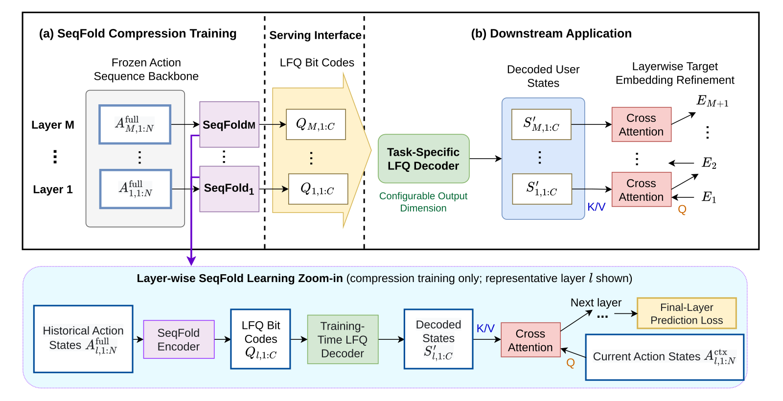
One action can write into several channels at once
The gate decides which channels an action writes into and how much. SeqFold gives each channel its own sigmoid instead of a softmax across the 64 channels.
The difference is whether one action can matter to several channels at once. Illustration: suppose two channels should both remember the action "add a stroller to cart". With sigmoids, the two channels can give 0.9 and 0.8. With a softmax, the weights of all 64 channels must sum to 1, so these two channels together get at most 1, roughly half each.
Each channel decides how long it remembers
Gating alone is not enough: once an action is written in, how much should it count as time passes? SeqFold makes each channel's state a weighted sum of all earlier actions, with weight . Here is how long ago that action happened, and is the decay rate this channel learns for itself.
Why not one global decay constant? Illustration: one channel keeps 0.9 after a year, which suits remembering a rare big purchase like a stroller; another keeps only 0.1 after a year, which suits remembering which phone cases are being compared right now. A single constant can only pick one.
This also shows how SeqFold differs from truncation. Truncation is a hard cut: actions before the last 64 get weight zero. Decay is soft: the stroller from three months ago still counts in a slowly decaying channel.
Finally each fusion vector becomes one 64-bit integer
After step 3, the state for one timestamp is 64 FP32 vectors of 256 dimensions per layer, 262,144 bytes in total. That is already much smaller than the full hidden states, but because it must be sent to several downstream systems and stored for every historical record, it is still too large.
LFQ (Lookup-Free Quantization) is quantization without a codebook lookup. The fusion vector first goes through RMSNorm, then the LFQ module assigns bits by sign and maps it to a 64-bit binary code, which fits exactly in one 64-bit unsigned integer. How a 256-dim vector becomes 64 bits (for example, whether it is projected first) is not specified in the paper.
So in the illustrative example, the 9 p.m. Tuesday search finally receives something like this (values illustrative):
user u, tau = Tue 21:00
layer 1: [0x9f3a12c4e8b07d51, 0x04ee7a90c13b62f8, ...]   64 uint64 in total
layer 2: [...]                                            64 in total
layer 3: [...]                                            64 in total
layer 4: [...]                                            64 in total
total 4 x 64 x 64 bits = 2,048 bytes
After receiving these 256 integers, a downstream system uses its own decoder to restore each code into a continuous vector whose size follows its budget, such as 32, 64, or 128. Its own targets (for example, the candidates for this search) then cross-attend over these 64 vectors. Because there are only 64 vectors, the cross-attention cost scales with the number of channels, not with 1,700 actions.
Update after every action, export only at requested timestamps
With the interface fixed, an engineering question remains: how to compute these timestamp states in batches. A direct tensor implementation computes a full state for every action prefix, a tensor of shape [batch, actions, channels, dims]. The authors' long-history benchmark uses 10,000 actions, 64 channels, and 256 dimensions, which is over 160 million floats per sample per layer, about 0.66 GB in FP32.
Yet downstream queries arrive at only a few timestamps. The authors separate "state update" from "state materialization": the first happens after every action, the second only when requested. The weighted sum above can be rewritten as a recurrence:
Here is the decay between the previous action and this one, is the gate weight, and is the action's hidden state. Illustration with scalars: the first action writes 2, so ; when the second arrives with and writes 4, , the same as the weighted sum. During the scan each channel only needs the one it holds, with no copy kept for every prefix.
A requested timestamp gets the state after the last action strictly before . In the illustrative example, if there is a click at 20:58 and the search is at 21:00, the export is the state after the 20:58 click. The authors wrote a fused Triton kernel that puts gating, decay, accumulation, and export into one chronological scan. The backward pass stores only final states and periodic FP32 checkpoints, then scans backwards to rebuild the intermediate states.
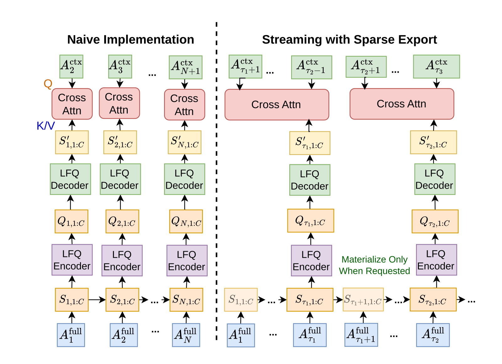
When training the compressor, the authors also use grouped export: a checkpoint is exported every actions, and queries between two checkpoints share the earlier one. Illustration: with , a query at action 150 sees the state after action 99, at most 100 actions late. This is a bounded visibility delay; actions 100 to 149 still update the recurrence, the query just cannot see them. Hoot says
Recurrent state: updated after every action
- After action 99
- S updated, a checkpoint is exported
- Actions 100 to 149
- S updated one by one, nothing exported
- Skipped actions
- None
The recurrence itself is not approximated
Query under grouped export (training, illustrative)
- Query at action 150
- reads the code after action 99
- It cannot see
- actions 100 to 149, 50 in all; they are already in S
- Worst case
- a query at action 199 still reads after action 99, 100 late
From action 200 on, queries read the checkpoint after action 199
Backfill and online serving: exact export
- Request
- the search at τ = 21:00
- Reads
- the state after the last action strictly before τ (the 20:58 click)
- Grouping delay
- None
Same scan, exporting only the requested timestamps
Illustrative: G = 100. Left: the recurrent state; middle: what a query reads under grouped export during training; right: exact export for backfill and online serving.
Source
paper §5.1 grouped export and bounded visibility delay; §5.2.1 Eq. (5); §5.2.2 Eqs. (6)–(7) (zero-based indexing, export set G−1, 2G−1, …); Figure 4 right panelThe baseline is a tensorized PyTorch implementation written with chunked cumprod/cumsum, which computes all prefixes first and then picks the requested ones. With batch size 10, bf16, and forward plus backward: exporting every prefix at 10,000 actions, the fused kernel takes 51.77 ms and the baseline 1014.48 ms, 19.6 times faster. Exporting only 1.56% of prefixes, the fused kernel drops to 18.45 ms and its peak memory from 35.0 GB to 2.0 GB, while the baseline stays around 1 second and about 20 GB. This shows that the sparser the export, the larger the gain from separating update and materialization, because the baseline must compute every prefix no matter how few are exported.
The last 64 actions take 262,144 bytes and are still 3.98% below 2 KB SeqFold
The main comparison uses query-level PR-AUC on the upstream action-prediction task; the data is proprietary, so only changes relative to SeqFold are reported. Each record takes the latest snapshot before its target event. All compared methods appeared above: full multi-layer hidden states, continuous fusion vectors without LFQ, window pooling (averaging every 32 or 64 neighboring actions into one), averaging the last layer into one vector, randomly sampling 64 actions, and the last 64 actions.
| Method | Metric change vs SeqFold | Bytes per snapshot |
|---|---|---|
| Full multi-layer hidden states | +2.11% | 6,963,200 (avg.) |
| Continuous fusion vectors (no LFQ) | +0.72% | 262,144 |
| SeqFold (fusion + LFQ) | 0 | 2,048 |
| 32-action window pooling | −1.10% | 217,600 (avg.) |
| 64-action window pooling | −1.38% | 108,800 (avg.) |
| Last layer averaged into one vector | −2.00% | 1,024 |
| Random sample of 64 actions | −2.37% | 262,144 |
| Last 64 actions | −3.98% | 262,144 |
The rows to look at are the three with equal storage. Continuous fusion vectors, 64 sampled actions, and the last 64 actions all take 262,144 bytes, yet their changes relative to SeqFold are +0.72%, −2.37%, and −3.98%. The latter two are below SeqFold, which takes only 2,048 bytes. This shows that at the same budget, summarizing the whole history with learned gates and decay pays off more than keeping a subset of raw actions.
At equal storage, what decides quality is how the whole history is summarized; choosing which raw actions to keep does worse.
The LFQ row answers what quantization costs: from continuous fusion to SeqFold, storage shrinks another 128 times and the metric drops 0.72%. Averaging the last layer into one vector takes only 1,024 bytes, half of SeqFold, but loses 2.00%; the authors' reading is that one vector cannot hold the many interests in such a long history.
How much truncation loses depends on the snapshot protocol here. The authors use it to model settings where signals from the most recent actions may be delayed or not yet final, and the last 64 actions depend most on exactly that stretch. The authors themselves note that results may differ under other online serving assumptions.
Ablation differences for channel count, fusion layers, and decay type
The ablations take the compressor's parts apart. Going from 64 channels down to 8 lowers the metric by 1.16%; going up to 128 adds only 0.08%, so 64 is the default. Compressing only the last layer is 0.97% below compressing all four, and adding a second and third layer narrows the gap to 0.52% and 0.44%. From this the authors infer that states from different depths give downstream complementary information.
The decay ablation uses no decay as its reference: fixed constants (0.3 or 0.6 remaining after one year) give −0.02% and +0.03%, and letting each channel learn its own decay rate gives +0.18%. These ablations use different references, so each difference only shows the effect of its own change and cannot be used to split credit for the overall result.
Code length also has a turning point. At 16 bits per code a snapshot needs only 512 bytes but loses 0.99%; 96 bits costs half again as much storage and is 0.05% lower. This shows that below 64 bits quantization still drops useful information and above it more bits bring no gain, so the authors take 64 bits.
The same codes go to search and QAC
The last experiment hands the codes to two real downstream tasks: search and QAC. Each learns its own decoder, with projection sizes 32, 64, and 128, and the control is the existing model with no SeqFold state at all. Search's primary metric rises by 0.24%, 0.49%, and 0.61% relative, and QAC's by 0.10%, 0.53%, and 0.60%. This shows that the same 2 KB code gives gains whatever size each downstream decodes it to, with most of the gain already at 64 dimensions. Because the control uses no state, these numbers answer whether the code helps, not whether it beats giving downstream the full states.
Back to the 9 p.m. Tuesday search. SeqFold's whole design rests on this: the search record needs only the 256 integers from before 9 p.m., so each of the 1,700 actions updates the accumulators as it arrives, but the result is written out only at the 9 p.m. timestamp.
How did this read for you?
Hoot made a note. Thanks for the feedback.

One tap, no sign-in; tap again to undo. Only anonymous counts are kept, never who you are.
Related papersMore from Paper Daily
 Personalization · 2026-11-11Query- and Candidate-Aware Long User Sequence Modeling for Sponsored Product Ranking in SearchWhen sponsored search ranking uses long-term behavior, the usual approach searches history for actions similar to the candidate product, which can miss history highly relevant to the current query but only loosely tied to the candidate. Beyond recent behavior, Wayfair retrieves one batch of long-term actions by candidate and another by query, then feeds them to a Transformer with two context toke…
 Personalization · 2026-08-03UxSID: Semantic-Aware User Interests Modeling for Ultra-Long SequenceDeep dive: UxSID: Semantic-Aware User Interests Modeling for Ultra-Long Sequence.
 Personalization · 2026-09-10Task-Blind No MORE: Multi-Task Information Flow in Unified Ranking BackbonesDeep dive: Task-Blind No MORE: Multi-Task Information Flow in Unified Ranking Backbones.
Discussion
Add experiment details, reproduction notes or a different take. Requires a GitHub sign-in.
Loading the discussion…