SHARE

Most production ranking models first squeeze the user's behavior sequence into a fixed vector and only then hand it to the feature-interaction module; once that is done, later interaction layers can no longer see which clicks or add-to-carts were involved. Taobao's HiRank keeps the behavior sequence alive through every layer of the backbone, and builds the queries that search long-term history from the user's recent behavior sequence rather than from static profile features such as age or gender. On Taobao homepage CVR prediction, against the strongest baseline at a similar parameter budget, GAUC rises from 0.7615 to 0.7801; in an online A/B test, orders per user rise 2.27% and GMV per user 2.86%.
Ranking teams should read this one, especially those merging behavior sequences and feature interaction into one backbone. The core idea in one sentence: the behavior sequence and the other features read from and write to each other in every layer, and at the end everything is compressed per traffic scenario into one compact vector, from which several distinct projections each take their own view for high-order interaction. I think the most valuable part is the comparison with OneTrans, HyFormer and MixFormer on the same features and data, plus the ablation that splits the gain across components; the theory told through "effective rank" reads more like an after-the-fact diagnostic and deserves caution.
What problem is it actually solving?
Take a Taobao homepage example (illustrative). Among a user's last 48 actions, three were looking at running shoes and one added sports socks to the cart; her purchase history over the past year is long, mostly baby products and kitchenware, plus two sportswear purchases. Now we need a CVR estimate for a running jacket.
| Approach (illustrative) | What queries long-term history | What it mostly finds | Problem |
|---|---|---|---|
| Profile-driven | Female, 30, high spender | Baby products, kitchenware | Users with similar profiles get nearly identical results |
| Candidate-driven | The running jacket itself | The two sportswear purchases | Sees only the candidate's angle and misses that she is getting ready to run |
| HiRank's interest query | Recent sequence: running shoes, sports socks in cart | Sportswear purchases and running-related browsing | Exactly the evidence we want |
The trouble with profile-driven queries is that profile features rarely change, so many users' query vectors crowd into a few directions. The paper quantifies this with effective rank (eRank): stack a batch of vectors into a matrix, check how evenly its singular values are spread, and convert that into "how many directions are really used". By hand: if four singular values are 4, 0, 0, 0, all information sits in one direction and the effective rank is 1; if all four are 1, it is 4. In HiRank's experiments, the input queries for long-term retrieval have a mean effective rank of only 24.52, rising to 54.88 after retrieval, which shows that retrieval driven by the sequence really gives different users more distinct representations.
The second problem is structural. In the usual encode-then-interact pipeline, a DIN-style sequence module first compresses behavior into one vector, and a DCNv2-style interaction module then crosses it with user, item and context features. Once the sequence is compressed into one vector, later interaction layers cannot go back for other evidence. The third problem comes from multiple scenarios: purchase feedback on the Taobao homepage is sparse (only 0.92% of homepage samples carry a purchase, per the paper), so the model trains on samples from the homepage, main search and dozens of smaller scenarios together, and a shared representation tends to blur the differences between them.
The pipeline
| Stage | Input | What it does | Output |
|---|---|---|---|
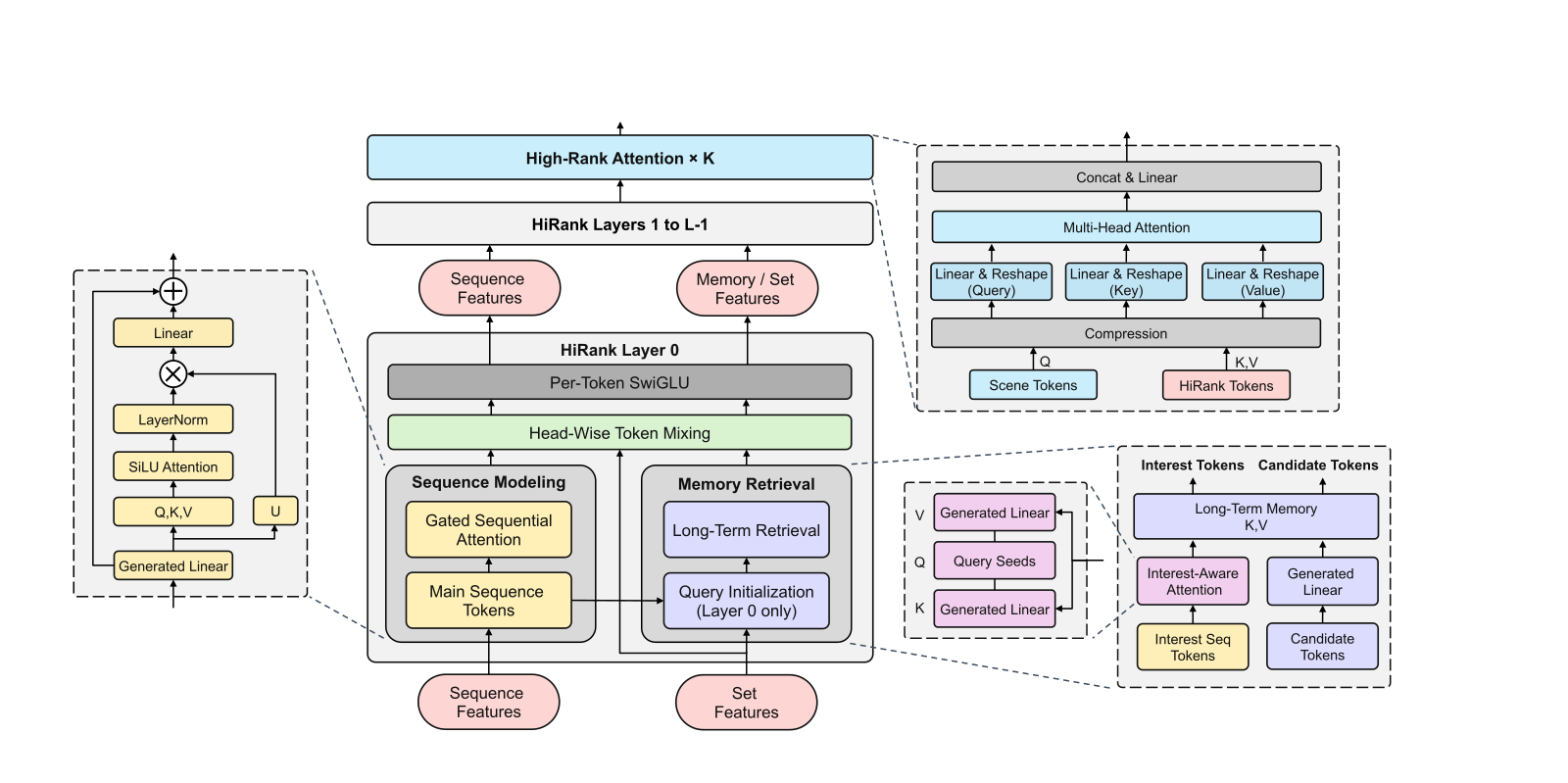
| Tokenization | User, item and context features; behavior sequences | Features are grouped by meaning, each group projected into a 256-d token; the main sequence keeps the latest 48 events; four long-term histories (clicks, add-to-carts, purchases and so on) are each projected into read-only memories | Feature tokens, main-sequence states, a candidate token, four long-term memories |
| HiRank layers (2) | All tokens from the previous step | Gated self-attention on the main sequence; two kinds of query read long-term memories; all tokens are mixed together | Updated sequence states, retrieval results and feature tokens |
| High-Rank Attention | All tokens from the last layer | Compress per scenario into one 1536-d vector, project it into 24 composite tokens, apply attention | One compact prediction state |
| Task towers | Prediction state | CVR as the main task, add-to-cart as auxiliary | Per-task probabilities |
The key division of labor: the main sequence says what the user is doing now, long-term memories say what she did before, and the interaction output decides what the next layer looks up. Let's take them apart.
Main sequence: why gated attention instead of DIN?
HiRank applies HSTU-style attention to the latest 48 actions. It differs from a standard Transformer in two places: attention weights use SiLU instead of softmax and are divided by the valid length, and the result is multiplied by a gate. Each query-key score goes through SiLU on its own to become a weight, without being compared to other positions.
Why not softmax? Take two users, one who looked at running shoes three times recently and one who looked once (illustrative): after softmax both could put nearly all weight on the running-shoe part, and the model cannot tell whose interest is stronger. SiLU does not require weights to sum to 1, but the aggregate is still divided by the main sequence's valid length; with equal valid lengths and comparable attention scores and value representations, more relevant contributions pointing in the same direction can increase the aggregate signal. The gate multiplies each position's own features with the aggregated history, letting the current action decide how much to take from the history.
The candidate item takes part too, but in a limited way: it reuses the keys and values this layer computed for the main sequence and reads them with its own query, but writes nothing back into the sequence during this attention read. Sharing user-side computation across candidates throughout the backbone requires the optional decoupled variant, whose mixing masks also block item-to-user feedback.
Long-term history: why two kinds of query?
Long-term histories are too long to put into the main sequence's self-attention, so HiRank treats them as read-only memories and searches them with queries. The two kinds of query each cover one side.
Interest queries come from the main sequence. In the first layer, a set of learnable seed vectors attends over the main sequence, producing several interest queries. These queries are split in advance into 4 groups, one per long-term history, and each group uses cross-attention to pull relevant behaviors from its own history only. At the same time, the candidate item itself acts as a query against each history, and the two sets of results complement each other. Back to the opening example: the seeds read "running shoes, sports socks in cart", so the resulting query leans toward sports and pulls out the two sportswear purchases.
Candidate queries come from the candidate item and read the same memories, answering "which of her past actions relate to this item". The two complement each other: one starts from the user, the other from the item.
There is also a loop between layers: after mixing in each layer, both retrieval results become the next layer's queries. What the first layer learns through interaction therefore shapes what the second layer looks up in long-term history. The memories never change; what changes is what you ask them.
Feature interaction: head-wise mixing, then per-token transforms
Once sequence states, both retrieval results, feature tokens and the candidate token are concatenated, the interaction layer works in two steps. The first borrows from RankMixer and TokenMixer-Large: split each token's 256 dimensions into 32 heads of 8 dimensions; then concatenate the first head of every token into a new token, the second head into another, and so on, pass each through a SwiGLU, and restore the original token layout. A small example by hand: 4 tokens of 4 dimensions split into 2 heads; after mixing, the first new token holds the first 2 dimensions of each of the 4 original tokens, 8 dimensions in total. This lets information from different sources interact within the same channel group. The second step gives each token its own SwiGLU with separate parameters to recombine its channels. Hoot says

Before: 4 tokens × 4 dims (2 heads)
- token A
- A1 A2 ‖ A3 A4
- token B
- B1 B2 ‖ B3 B4
- token C
- C1 C2 ‖ C3 C4
- token D
- D1 D2 ‖ D3 D4
Each token holds only its own source's information.
After head-wise mixing: 2 new tokens × 8 dims
- New token 1 (head 1)
- A1 A2 B1 B2 C1 C2 D1 D2
- New token 2 (head 2)
- A3 A4 B3 B4 C3 C4 D3 D4
- A SwiGLU each
- then back to 4 tokens
After restoring, every head of every token has interacted with the same head of the others.
Left: one row per original token (A1 A2 is its head 1, A3 A4 its head 2). Right: one row per mixed token. In the real model each token has 256 dims in 32 heads of 8. Source: paper's interaction layer (after RankMixer / TokenMixer-Large): 256 dims split into 32 heads of 8, regrouped by head, a SwiGLU each, then restored; the 4-token example is the article's
Why not plain self-attention over all tokens? The paper's reasons: recommendation features are highly heterogeneous, single-head attention output cannot exceed the rank of the values, and pure attention stacks tend to make tokens increasingly alike; OneTrans's ablations also show that keeping every token in every layer adds computation without reliably helping. Head-wise mixing learns no attention weights, is cheap, and still guarantees every token receives information from all others.
High-Rank Attention: compress per scenario, then look from several angles
The backbone outputs many tokens, and high-order attention on all of them is both expensive and noisy. HiRank first compresses with scene tokens: it builds a few queries from the sample's traffic scenario (homepage, main search or another) and cross-attends over all last-layer tokens, flattening the result into one compact 1536-d vector. Homepage and search samples thus pull different evidence from the same pile of tokens; this is how it handles multiple scenarios.
Then come Hiformer-style composite projections: three independently parameterized composite projections read the full 1536-d vector and separately produce queries, keys and values, with 24 tokens of 256 dimensions in each set; multi-head attention then uses these three sets. The 24 attention outputs of 256 dimensions are concatenated into one 6144-d vector, which a linear layer maps back to 1536 dimensions and adds to the compact vector as a residual. Each task, such as click or conversion, has its own small MLP tower that reads this updated vector and outputs its probability. Why not just cut the 1536 dimensions into 24 slices? With slices, each token sees only part of the information; composite projections let every token see all of it, each from a different angle. The paper's effective-rank diagnostic shows that across this step the mean effective rank goes from 228.58 to 224.09, a drop of only 1.96%, meaning the high-order interaction does not squeeze the representation into a few directions.
Results
Offline data are Taobao-wide CVR samples, about 2.4 billion impressions a day, about 438 million of them on the homepage. All compared models use the same features, histories and training data, tuned on validation CVR AUC. The table below is taken from the paper's Table 2:
| Model | Homepage AUC | Homepage GAUC | Main search AUC | Params (M) | GFLOPs per candidate |
|---|---|---|---|---|---|
| DCNv2 + DIN (production base) | 0.9136 | 0.7294 | 0.8748 | 36.98 | 0.428 |
| RankMixer + DIN | 0.9143 | 0.7473 | 0.8755 | 350.15 | 1.002 |
| OneTrans | 0.9154 | 0.7592 | 0.8759 | 345.40 | 1.768 |
| HyFormer | 0.9148 | 0.7615 | 0.8758 | 344.40 | 1.280 |
| MDL (multi-scenario) | 0.9147 | 0.7439 | 0.8756 | 343.62 | 0.990 |
| HiRank | 0.9163 | 0.7801 | 0.8764 | 299.04 | 1.530 |
Homepage GAUC beats the strongest baseline, HyFormer, by 0.0186, while global AUC beats OneTrans by only 0.0009. The gap says HiRank's gain lies mostly in "which item to show this user first", which is exactly what retrieval driven by the user's own sequence is meant to improve. On main-search traffic (the other half of the paper's Table 2), HiRank's GAUC beats that scenario's strongest baseline by only 0.0009 and its AUC by 0.0005, so the design helps homepage recommendation far more than search, where the query is a strong signal and user history adds less. On cost, HiRank has 46M fewer parameters than OneTrans and about 13% less computation per candidate.
The ablation (paper Table 3, homepage CVR) splits the gain across components:
| Component removed | AUC | GAUC |
|---|---|---|
| Gated attention (replaced by DIN) | 0.9160 | 0.7623 |
| Two-query retrieval (replaced by candidate-only DIN) | 0.9159 | 0.7591 |
| Feature interaction | 0.9158 | 0.7714 |
| High-Rank Attention | 0.9154 | 0.7685 |
| Both feature interaction and High-Rank Attention | 0.9143 | 0.7312 |
| Full HiRank | 0.9163 | 0.7801 |
Two-query retrieval has the clearest contribution: querying long-term history with the candidate alone drops GAUC by 0.021, close to HiRank's entire lead over the strongest baseline. Removing interaction and High-Rank Attention together drops GAUC to 0.7312, almost back to the production base, supporting the complementary roles of behavioral modeling and feature interaction in this model.
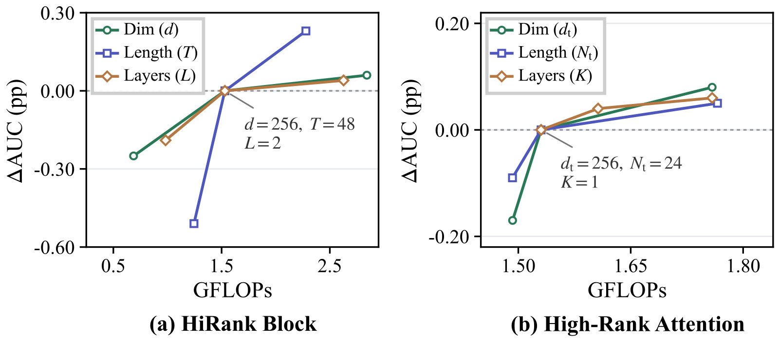
The scaling study gives a very practical signal: in this architecture, a longer main sequence pays off far more than going wider or deeper. That fits the design in which the main sequence generates the retrieval queries; the longer the sequence, the more accurate the interest queries.
The online A/B test ran on Taobao homepage traffic with user-level buckets against the production ranker: orders per user up 2.27% (p<0.01), GMV per user up 2.86% (p<0.05), daily purchasing users up 2.13%. Page views rose only 0.45% while orders per thousand impressions rose 1.81%, so the growth comes mostly from conversion efficiency rather than from showing more items.
Where I think it falls short
First, the effective-rank argument is correlation, not causation. The paper shows effective rank rising from 24.52 to 54.88 across retrieval, but runs no control such as "lower the effective rank and see whether accuracy drops", nor compares effective rank against AUC across architectures. The title leads with effective rank, yet the evidence comes mainly from the ablation table.
Second, serving cost is unclear. The paper proposes a decoupled version in which candidates in one request share user-side computation, but reports neither its offline accuracy nor its online latency, and does not say which version ran in the A/B test. At 1.530 GFLOPs per candidate, HiRank costs 3.6 times the production base's 0.428; for teams without request-level batching, that gap is decisive.
Third, all baselines were reproduced by the authors on their own data. The OneTrans and HyFormer papers each reported solid online results, yet here the newer baselines differ in homepage AUC by at most 0.0016, and outsiders cannot judge whether reproduction and tuning effort was equal. On main search, HiRank's global AUC beats the strongest baseline by only 0.0005, a reminder that its gains depend heavily on the scenario.
How a recommendation team could try it
- First test where the long-term retrieval query comes from: keep the current model and only replace the query that searches long-term history, from profile features or the candidate item, with learnable seed vectors reading the recent sequence; check whether GAUC improves clearly. The related ablation replaces the full complementary retrieval module with candidate-only DIN, lowering GAUC from 0.7801 to 0.7591 and measuring the effect of the full replacement.
- At the same time, measure the effective rank of the query vectors. If the current queries have a low effective rank, different users are retrieving nearly the same things, and there is more room to gain.
- If it helps, add the layer-to-layer loop: let the interaction output become the next layer's retrieval query, compare one layer against two, and record computation per candidate.
- Consider scenario compression and composite projections last. With mixed multi-scenario training, first add only scene-token compression and check whether each scenario's GAUC improves on its own; in parallel, try a longer main sequence first, since the paper finds it the cheapest way to scale.
Verdict
Letting a user's recent behavior decide what to look up in long-term history separates users better than letting static profiles or the candidate item do it; that is the part of HiRank most worth borrowing. The full architecture is computationally heavy and suits teams that already run large ranking models.
| Dimension | Assessment |
|---|---|
| Problem importance | High. Fusing sequences with feature interaction and training across scenarios are common challenges in large-scale ranking |
| Method novelty | Medium. Most components come from HSTU, RankMixer and Hiformer; the new parts are sequence-generated retrieval queries and the layer-to-layer loop |
| Experimental evidence | Medium-high. Real Taobao data, same-condition comparison with several recent baselines, ablations and an online A/B; the effective-rank part is only a diagnostic |
| Engineering cost | High. Computation per candidate is 3.6 times the production base, and the decoupled version's accuracy and latency are not reported |
| Worth trying | Try the sequence-generated retrieval query; adopt the full architecture according to your compute budget |
How did this read for you?
Hoot made a note. Thanks for the feedback.

One tap, no sign-in; tap again to undo. Only anonymous counts are kept, never who you are.
Discussion
Add experiment details, reproduction notes or a different take. Requires a GitHub sign-in.
Loading the discussion…