Contents · 10 sections
1What problem is it actually solving?2Pipeline overview: one fix per stage3Commercial ID: the last code is split by bid tier4How the value head is trained: the hardest step in the paper5Generation as ranking: add the two scores at every step6A per-request tree: no beam width wasted on unservable ads7Experiments: components added offline step by step, versions shipped online one by one8Limitations as I see them9How a generative ads team could try it10VerdictSHARE

Teams working on generative recommendation, especially those who want to bring it to ads, should read this paper, because it breaks the conflict "the most probable item is not the most profitable one" into three concrete leaks and gives a deployable fix for each. The core idea in one sentence: the last digit of an ad's ID is no longer split by content similarity but by "commercial conditions plus bid tier"; at every decoding step the model adds a learned commercial value score to the generation score, and it searches only among ads that can actually be served for this request. On Tencent's industrial offline ads data, HR@100 improves 37.04% relative to the baseline; in a 5-day online test on 20% of WeChat Channels traffic, GMV rises 1.50%. With a per-request trie, a beam of width 300 returns 300 valid ads instead of 48, and the average bid rises from 1.29 to 11.44.
What problem is it actually solving?
In generative recommendation each item has an SID, and the model reads the user's history and generates the SID one position at a time; the generated SID maps back to the item to recommend. The SIDs here have three positions with a 2048-entry vocabulary each. Which SID wins is decided by generation probability. Below, an SID is also called an "ID" or "code".
Ads are different. Besides whether the user likes the ad, it matters how much commercial return the ad brings for this request, which depends on bid, ROI target, eCPM and so on. The paper traces value loss to three stages:
| Stage | What goes wrong | Illustrative example |
|---|---|---|
| ID | IDs are split by content similarity, so ads with very different bids share the same ID | Ten tower-defense game ads share one ID, with bids from 0.15 to 0.24 |
| Decoding | Generation looks only at probability, so a high-value ad with a low-probability prefix is pruned early in beam search | A high-bid ad's first code ranks 301st and never comes back |
| Serving | Search runs over the global ID space, ignoring which ads this request can serve | Most of the beam is ads with exhausted budgets or mismatched targeting, filtered out at the end |
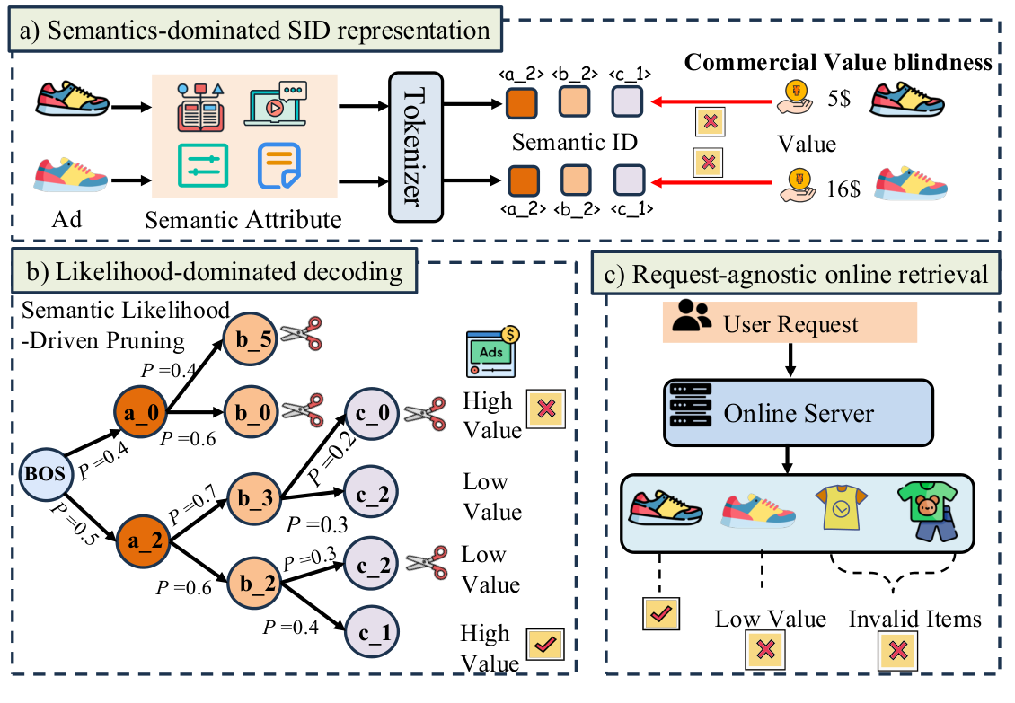
This shows the problem is not one weak module: every step of the pipeline assumes "more probable is better", so each stage needs its own fix.
Pipeline overview: one fix per stage
The paper's method is called UniVA, with one component per stage:
| Component | Stage | What it does |
|---|---|---|
| Commercial ID (CSID) | ID | Keep the first two semantic codes; replace the last with a "commercial conditions plus bid tier" code |
| Generation-as-ranking decoder | Decoding | One decoder with two heads: one gives generation scores, the other gives a commercial value score per candidate code; the two are added during decoding |
| Request-constrained serving | Serving | Build, for each request, a prefix tree that contains only servable ads; beam search walks only on that tree |
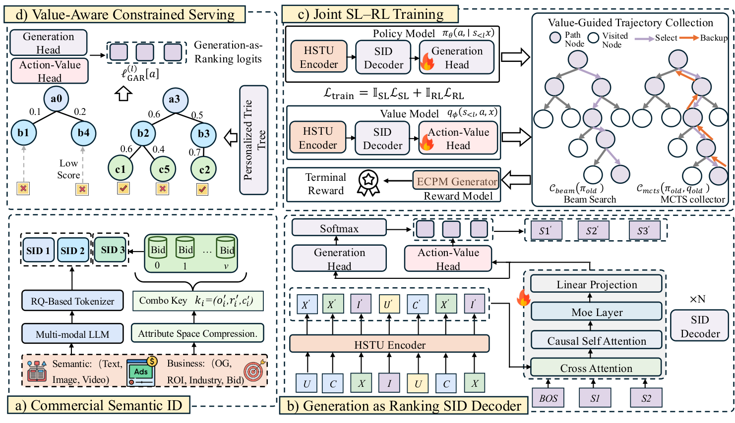
Commercial ID: the last code is split by bid tier
Why change the ID? If ads with very different bids share a full ID, the model cannot tell them apart at the ID level, and no amount of value learning later can fix that.
The commercial ID is built in two steps. The first step compresses commercial attributes, because their raw values are too many and too sparse: optimization goal, ROI target and industry each keep their frequent values and merge the long tail. On the industrial data, optimization goal becomes 25 categories, ROI 8, and industry 10. The three together form a "combination key", and keys with fewer than 3 samples are merged into a fallback key.
The second step splits each key into bid tiers. Key gets tiers with equal sample counts per tier (equal-frequency binning); the total number of tiers is at most 2048, and each key gets between 3 and 25 tiers. The tier counts are chosen by one objective: make usage of the last code as even as possible, i.e. maximize , where is the key's sample share.
A small hand-computed example: three keys have sample shares 50%, 30% and 20%, there are only 12 tiers in total, and each key needs at least 3. The split (6, 3, 3) scores about 2.475, while (5, 4, 3) scores about 2.470. So the dense key gets more tiers, and the codes are used 8.3%, 10% and 6.7% of the time, which is fairly even. This means dense commercial scenarios get finer bid splits, while sparse ones do not create codes almost nobody uses.
A quick upper bound follows too: with at least 3 tiers per key and a budget of 2048, at most about 682 keys can be retained (my calculation from the paper's settings). The final commercial ID uses 1,939 codes.
One full ID may still hold several ads, so serving has to pick one: it first takes the ads this request can serve, then picks the one with the highest bid.
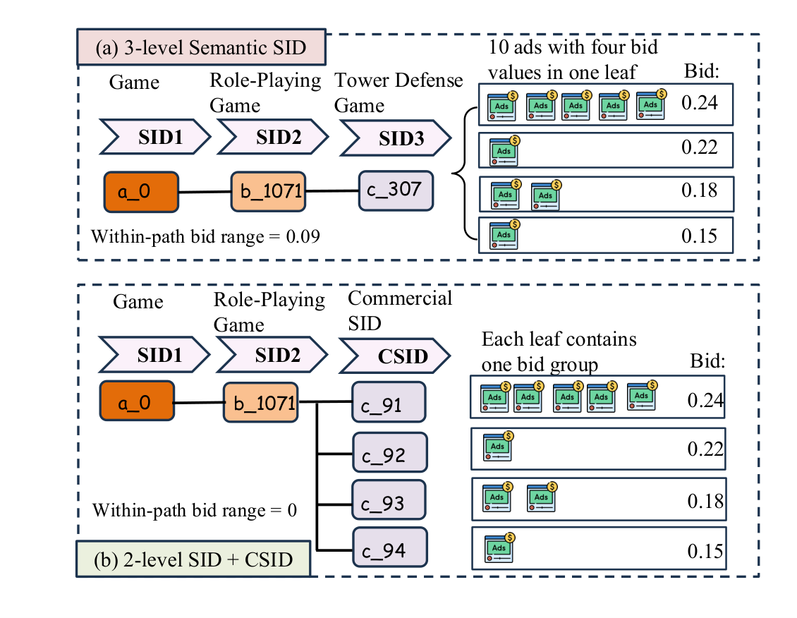
On the effect: the paper samples about 690,000 ads and uses conditional R², i.e. among ads sharing the first two codes, the share of total bid variation that lies between groups formed by the last code. Replacing the last code with the commercial code raises this share from 57.6% to 99.2%; the same calculation for expected ROI goes from 51.2% to 89.9%; bid dispersion within a full path mostly drops by about an order of magnitude. This shows ads under the same ID now have consistent commercial value, so the decoder can tell expensive from cheap by ID.
How the value head is trained: the hardest step in the paper
Why a second head? The commercial ID makes value distinguishable, but which code is worth more for this request still depends on the user and context. UniVA adds an "action-value head" to the decoder that outputs a score for every candidate code in the vocabulary, meaning "how much commercial return you end up with if you pick this code after the current prefix".
Training alternates two kinds of batches. Supervised batches are ordinary next-code prediction, which keeps generated codes valid and relevant. Reinforcement learning batches go as follows:
- Collect trajectories: at the start of each round, freeze a copy of the current model, written as the old policy and old value head . For each request, first run beam search with the old policy to get the high-probability complete codes; then run a Monte Carlo tree search (MCTS), used only offline, that allocates extra search to prefixes with high value scores. The complete codes from both together are this request's trajectory set.
- Score: each complete code resolves to a concrete ad by the same bid-priority rule used online, i.e. the highest-bid ad among those this request can serve, and that ad goes to an offline simulator that computes eCPM. The simulator's click-rate and conversion-rate predictors are copied from the production ranking system.
- Normalize within the request: subtract the mean and divide by the standard deviation over the trajectories of the same request, so that rewards are comparable across requests. For example, if four trajectories have eCPM 10, 20, 30 and 40, the mean is 25 and the standard deviation about 11.18, so the normalized values are -1.34, -0.45, 0.45 and 1.34. The reward is given only at the last code; earlier positions get 0.
- Update: the generation head is updated with PPO, and the value head, for the code chosen at each step, regresses to a target computed from that trajectory's reward.
At each node (that is, a prefix), MCTS picks, among valid next codes, the that maximizes . is the visit count, and the second term gives branches with high prior probability that have rarely been visited a chance to be explored. has two cases: for an edge no complete trajectory has passed through yet, it is simply the old value head's score ; once visited, it becomes the mean normalized reward (step 3) of the complete trajectories that passed through that edge. For this action-value-guided MCTS trajectory collection, the paper does not state where the search gets the request-level reward mean and standard deviation needed for the backup before the search ends, even though those statistics are defined over the final collected trajectory set, so a reimplementation has to choose its own approach. For example, if two trajectories passed an edge with rewards 1.34 and -0.45, its is 0.445.
The key is the target in step 4. The paper first uses the old value head to build a baseline at each position: , the expectation of over valid codes under the old policy. The valid code set here is the same as in search: it depends on the current request and the prefix generated so far, and probabilities are renormalized within that set; only complete trajectories that resolve to a servable ad are scored, which the paper calls feasible trajectories. After the last position, . It then applies generalized advantage estimation (GAE) position by position: , advantage , and target . is PPO's advantage and is the value head's regression target; neither passes gradients back.
A hand-computed three-position trajectory, taking for illustration: baselines 0.2, 0.5 and 0.9, final reward 1.34. Then is 0.3, 0.4 and 0.44, the advantages are 1.14, 0.84 and 0.44, and adding the baselines back gives a target of 1.34 at all three positions. When is below 1, earlier positions partly borrow the old value estimates of later positions instead of depending entirely on the final reward. This means (prefix, code) learns how high, relative to this request, the eCPM of the ad you finally land on is if you pick this code after this prefix.
So the value head has three uses with one set of parameters: it is PPO's baseline in training; in offline MCTS it estimates the value of branches not yet visited; and in online decoding it takes part in ranking directly.
Generation as ranking: add the two scores at every step
Online, at each position, the outputs of the two heads are added: , where is a per-position coefficient chosen on validation data and then fixed. With this falls back to plain generation.
A hand-computed step: candidate code A has generation score 2.0 and value score 0.1; B has 1.5 and 0.8. On generation score alone, A leads; with , A gets 2.1 and B gets 2.3, so B overtakes. This means a branch with a modest-probability prefix that leads to high-value ads can be kept before it is pruned.
A per-request tree: no beam width wasted on unservable ads
Why constrain per request? Each request can serve different ads: targeting, exhausted budgets, frequency caps and content compliance each rule some out. Searching the global ID space first and filtering afterwards wastes most of the beam.
How it works: every day about 5 million creatives are sampled from the full library, and a global prefix tree is built over their full IDs, with creatives hanging on the leaves. When a request arrives, the servable set is filtered by targeting, ad status and creative rules; leaves with no servable creative are removed, and internal nodes left without children are removed all the way up, leaving a tree for this request alone. During decoding, the fused score from the previous section gets the mask added, with codes not on the tree set to negative infinity, and then goes through softmax and a log; beam search ranks prefixes by the sum of these log probabilities over positions.
The paper compares with a beam of width 300: searching globally and then filtering leaves only 48 valid paths; searching on the tree keeps all 300 valid, and the average bid rises from 1.29 to 11.44. This shows that with a fixed beam width, pruning unservable branches early hands the slots to ads that are servable and bid higher.
Experiments: components added offline step by step, versions shipped online one by one
The industrial dataset comes from Tencent's mixed traffic, where ads and organic content are served together, split 80/20 into training and test. The baseline is GPR, an industrial generative ads model that already uses commercial signals in training and decoding. The main offline metric is HR@100; the table below adds components step by step, with parameters and compute counting only the decoder:
| Configuration | Params | Compute | HR@100 relative gain |
|---|---|---|---|
| Base: GPR encoder plus ID decoder | 3M | 4.1G | 0 |
| Add commercial ID | 3M | 4.1G | +5.78% |
| Deeper decoder (4 independent layers) | 7M | 7.1G | +6.10% |
| Switch to recursive parameter sharing (MoR) | 5M | 7.1G | +13.56% |
| Add sparse experts (MoE) | 60M | 8.5G | +18.40% |
| Add eCPM reinforcement learning and generation-as-ranking | 62M | 8.5G | +32.01% |
| Full (more recursion, 16 of 64 experts) | 80M | 23.2G | +37.04% |
In the MoR row the decoder is an input layer, one shared middle layer and an output layer; the middle layer runs twice with the same parameters, so effective depth is still four layers while parameters drop from 7M to 5M. The full version runs the middle layer four times, for six effective layers. The sparse-expert row replaces the feed-forward layer with 16 routed experts plus one always-on shared expert, and each code activates only the top 4 routed experts, so parameters grow to 60M while compute only goes from 7.1G to 8.5G. The commercial ID adds 5.78% at no extra compute; reinforcement learning plus generation-as-ranking gives the largest jump, from 18.40% to 32.01%, with almost no change in parameters or compute. But that row adds PPO training and value-score fusion at decoding together, so the table cannot split their shares.
ID design comparison (HR@100, raw values from the table):
| ID configuration | HR@100 |
|---|---|
| 3 semantic levels, 2048 each | 3.23 |
| 3 semantic levels, 8192 each | 4.03 |
| 2 semantic levels (2048) plus commercial ID | 4.20 |
| 2 semantic levels (8192) plus commercial ID | 3.84 |
The commercial ID works best with 2048-way semantic levels; with 8192 it is worse than pure semantic IDs. The paper's explanation is that the commercial vocabulary is fixed at 2048, which matches 2048-way semantic levels, while replacing an 8192-way semantic level loses more fine-grained splitting. This shows the commercial ID is not "more is better"; it has to match the size of the semantic levels.
The public datasets (Amazon Industrial and Office) have no bids or other commercial attributes, so no commercial ID is built and ratings serve as the value signal. UniVA ranks first on every metric, 1.5% to 8.4% above the strongest baseline, e.g. Office HR@3 from 0.1217 to 0.1319. This shows the value head and decoder are usable beyond ads, but the gains are much smaller than on the industrial data.
The online test ran from March 7 to 11, 2026 on 20% of traffic, with all four versions compared against the same production baseline. GMV(normal) uses the same attribution as GMV but excludes ads whose campaigns optimize an ROI target, in order to reduce noise from traffic shifts in those campaigns:
| Version | GMV | GMV(normal) |
|---|---|---|
| V0: semantic ID plus GRPO | +0.22% | +0.45% |
| V1: V0 with a larger decoder | +0.36% | +0.77% |
| V2: V1 with the commercial ID | +1.03% | +1.17% |
| V3: full UniVA (PPO plus value head plus generation-as-ranking) | +1.50% | +1.42% |
The largest online jump comes from switching to the commercial ID (V1 to V2, 0.67 more points of GMV), and the value head with generation-as-ranking adds another 0.47 points (my calculation from the table). This shows the ID-level change matters just as much online.
Limitations as I see them
First, reinforcement learning and generation-as-ranking are not separated. The offline jump from 18.40% to 32.01% adds PPO training and value-score fusion at decoding together, and online V3 also ships both. So readers cannot tell how much the value head contributes to online ranking. The full version then raises compute from 8.5G to 23.2G, about 2.7 times, for only 5 more points (my calculation from the table).
Second, the value signal comes from a simulator, yet the step-by-step ablation only looks at hit rate. The RL reward comes from a simulator that copies the production click-rate and conversion-rate models, while the main offline table reports HR@100 (next-interaction prediction); the GMV-weighted ValueHR appears only in Figure 3 to compare ID designs, not in the step-by-step ablation. ValueHR@K is computed on the GMV-weighted next-conversion test set: take the requests whose true converted ad lands in the top K candidates, sum their GMV, and divide by the total GMV of all requests. Online ran only 5 days, and GMV(normal) gains just 0.25 more points from V2 to V3, and 5 days of data cannot show whether that part of the gain holds.
Third, the commercial ID is built offline, while bids change every day. An ad that changes its bid may move to another tier, its last code changes, and what the model learned about that code drifts. The paper's appendix also admits incremental ID updates are unsolved. Online, each request filters about 5 million creatives to build a tree, then runs a beam of width 300 with a 23.2G-compute decoder; Table 4 reports only GMV, so in my reading this cost is the first thing to measure before launch.
How a generative ads team could try it
- Quantify the problem first: measure the standard deviation and range of bids among ads sharing a full ID under the current scheme. If bids under one ID differ several-fold, the ID itself cannot tell value apart.
- Do the cheapest step first: keep the first two semantic levels and rebuild the last level as "compressed commercial attributes plus equal-frequency bid tiers", with tiers allocated by sample share. Compare HR and bid dispersion offline without changing the model.
- Then add the per-request prefix tree: in offline replay, compare valid path counts for "search then filter" against "search on the tree", and measure tree-building time.
- Add the value head last: use it first only in offline MCTS and PPO, check that value scores correlate with simulator eCPM, then tune the fusion coefficient on validation data and launch from a small value.
- Rebuild the commercial ID regularly and monitor the share of ads whose ID moves because of bid changes.
Verdict
| Dimension | Assessment |
|---|---|
| Problem importance | High. As generative recommendation enters ads, the conflict between commercial value and generation probability cannot be avoided |
| Method novelty | Medium-high. Encoding bid tiers directly into the ID, and using one value head across training, search and online ranking, is a fairly new combination |
| Evidence | Medium. Both the step-by-step offline ablation and the version-by-version online comparison exist, and the commercial ID analysis is solid; but RL and value fusion are not separated, the online test is 5 days, and there is no latency data |
| Engineering cost | High. Needs an offline simulator, MCTS collection and per-request tree building; the full decoder costs 23.2G compute |
| Worth trying | Yes. Start with the commercial ID and the prefix-tree constraint; neither needs RL, and in the online table the commercial ID step alone accounts for almost half of the GMV gain |
How did this read for you?
Hoot made a note. Thanks for the feedback.

One tap, no sign-in; tap again to undo. Only anonymous counts are kept, never who you are.
Related papersMore from Paper Daily
 Generative · 2026-10-15WeGR: Unified Generative Retrieval for Industrial Search Systems in WeChatDeep dive: WeGR: Unified Generative Retrieval for Industrial Search Systems in WeChat.
 Generative · 2026-11-02Towards Reliable, Scalable, and Value-Aligned Generative Recommendation for Large-Scale AdvertisingKuaishou made three changes to GR4AD, its deployed generative ad retrieval system, and the result, GR4AD-X, raises online ad revenue by a cumulative 3.07% over GR4AD. All three target the same mismatch: the model picks ads by generation probability, while the platform cares about revenue. The top ten ads by generation probability and the top ten by eCPM barely overlap, with a hit rate of only abo…
 Generative · 2026-11-05SPADE: Spatiotemporal Preference Alignment and Diversity Enhancement for Local SearchThe homepage of a local-services app must generate a few queries out of millions of possibilities, with no two alike, matching where the user is right now. At the input, the user's exact coordinate and the current hour are encoded as vectors and added in. Offline, HR@5 is 5.6% higher (relative) than the strongest generative baseline, and the average distance from the user to the recommended shops…
Discussion
Add experiment details, reproduction notes or a different take. Requires a GitHub sign-in.
Loading the discussion…