Contents · 8 sections
1A few terms first2How far to predict: about one second3Why executing fewer steps often does not help4Walking through it: the same red cube, four ways5Lower latency or smoother joins: which helps more6Change the model, or change how it is executed7What this means for people building robot policies8LimitationsSHARE

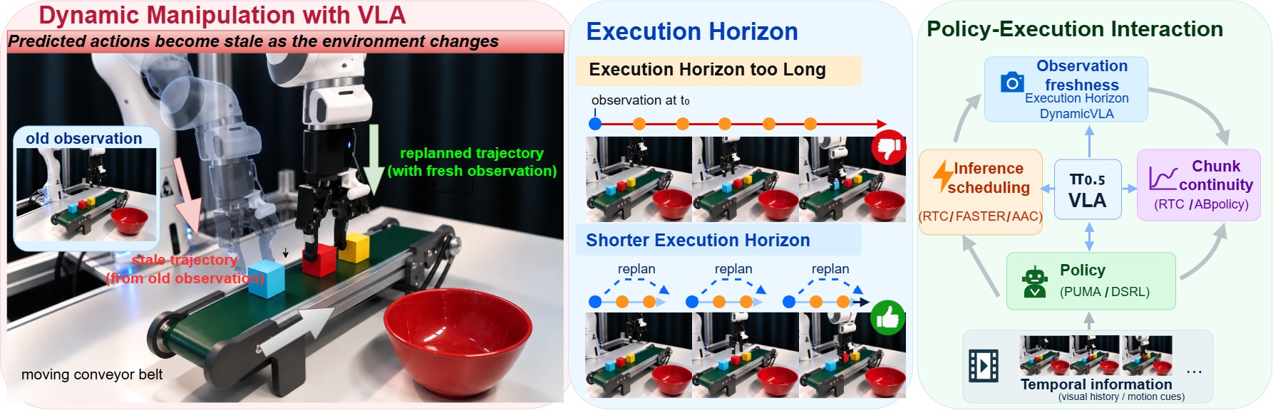
The cube has already ridden away on the belt, and the arm is still reaching for where it used to be: what limits how fast a VLA reactsA conveyor belt moves right at 5 centimeters per second, carrying three cubes of different colors. The robot arm has to pick out the red one and drop it into a bowl next to the belt.
The arm looks at the scene, the model computes the next second of motion in one go, and the arm carries it out. Halfway through, the red cube has already moved several centimeters to the right, and the arm is still reaching toward where the cube used to be.
Many of today's VLA models (large models that look at images, take an instruction, and output robot actions directly) work this way: they predict a whole stretch of future actions at once, called an action chunk. When nothing moves, this saves inference and keeps the motion smooth. When objects move, the chunk goes stale before it finishes.
This paper from the Karlsruhe Institute of Technology (KIT) takes a pretrained π0.5 and asks a practical question: how do you make it react faster in dynamic scenes? There are several families of fixes. One executes fewer steps before looking again. One overlaps inference with motion so the robot never stops to wait. One gets the first new action out sooner. One makes the new chunk join the old one smoothly. Others add motion information to the model or fine-tune it with reinforcement learning. The authors put these methods into one π0.5 framework and compare them on two dynamic simulation benchmarks and three real-robot tasks. The findings: predicting about one second ahead works best; executing fewer steps helps more with asynchronous inference; and among the methods tested, the highest success came from a method that keeps chunks continuous, and a lower-latency method did not beat another continuity method. The biggest surprise is on the conveyor task, where the same model with no training at all, changing only how many steps it executes per chunk, matches the success rate after reinforcement learning fine-tuning. How fast a robot reacts depends on how it executes as much as on the policy; these results come from π0.5 and a small set of tasks, with only 15 to 20 real-robot trials per setting.
A few terms first
Each time the model looks at the scene, it outputs an action chunk of H actions, where H is the prediction horizon. The arm does not have to execute all H actions. It can execute only the first s, then look again and predict again, and s is the execution horizon. H decides how far ahead the model plans, and s decides how much the arm does before it looks again.
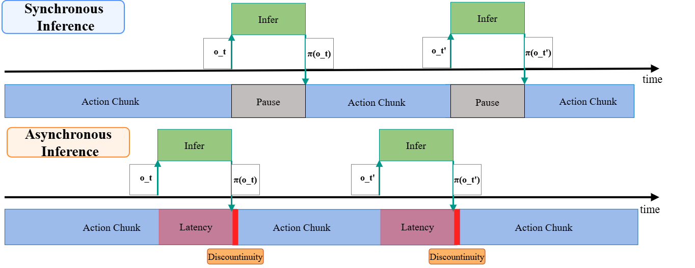
Synchronous execution means the arm finishes its s steps, stops, waits for the model to produce the next chunk, and then moves on. Asynchronous execution means that while the arm is still executing the current chunk, the model is already computing the next one from a new image, so the arm does not stop.
How old is the image behind the action the arm is executing right now? The paper calls this the observation age. The older the observation, the farther the object has moved from where the image showed it.
How far to predict: about one second
The authors first trained models with different prediction horizons. On DOM (a pick-and-place simulation benchmark in which the object is pushed into motion), the best was 25 steps. On the two tasks from DOMINO (another dynamic manipulation simulation benchmark), the best was 30 steps. The two simulators run at 25 and 30 control steps per second, so both optimal values come out to exactly one second of motion.
On this basis, the authors recommend in their conclusion choosing the prediction horizon in seconds.
Why executing fewer steps often does not help
Intuitively, a smaller s means the arm looks at fresh images more often, so it should react faster. The experiments say: not necessarily.
On the real conveyor task with s at 10, synchronous π0.5 and PUMA (covered later; it adds motion information to the model) succeed only 20% of the time, while the asynchronous methods reach 60% to 75%. This shows that with the same rate of looking, every 10 steps, synchronous and asynchronous execution can differ by more than a factor of three.
On DOM, as the same model's s gets smaller, the gap between synchronous and asynchronous execution keeps growing.
The cause is the stop in synchronous execution. A smaller s means more chunks, and so more stops to wait for inference. During each stop the arm stands still while the object keeps moving. With asynchronous execution, the next chunk starts computing while the current chunk is still running. As long as inference finishes within the time it takes to execute those s steps, a smaller s adds no waiting. RTC (Real-Time Chunking), covered later, sets the minimum execution horizon to the number of steps that the inference delay corresponds to.
Walking through it: the same red cube, four ways
Here is a walk-through on the fast conveyor setting. The belt speed of 5 centimeters per second, the action rate of 20 per second, and the 20-action prediction (exactly one second) all come from the paper. Inference time is taken as 0.3 seconds. That number is illustrative, based on the paper's Table 5, where synchronous π0.5 on an A100 takes 0.26 to 0.30 seconds to deliver its first action.
Step one: synchronous, s at 10. The arm takes a picture and then stops to wait 0.3 seconds, so the cube first moves 5 × 0.3 = 1.5 centimeters. After the actions arrive, the arm executes 10 steps, which takes 10 ÷ 20 = 0.5 seconds, and the cube moves another 2.5 centimeters. This means that by the last action of this chunk, the picture behind it is 0.8 seconds old, and the cube is 4 centimeters from where the picture showed it.
Step two: synchronous, with s cut to 5. Each round becomes 0.3 seconds of standing and 0.25 seconds of moving, so the observation age drops to 0.55 seconds and the cube's offset drops to about 2.8 centimeters. The cost is that the arm stands still 0.3 ÷ 0.55 of the time, more than half. The whole grasp is cut into more pieces, and every piece starts with a stop.
Step three: switch to asynchronous, still with s at 5. The model computes the next chunk while the arm moves, and the arm no longer stops. In the paper's Table 6, asynchronous π0.5 on the conveyor gets its first action in about 0.145 seconds. But the new chunk is computed from a picture taken 0.145 seconds earlier, so its first action does not necessarily start exactly where the arm is now. If it is far off, the arm has to jump. That jump is the red discontinuity in the figure.
Step four: raise the action rate from 20 to 30 per second. The same 10 actions now take 10 ÷ 30 ≈ 0.33 seconds instead of 0.5, so the cube moves only about 1.7 centimeters during the chunk instead of 2.5. In the paper, after raising the rate to 30 on the fast setting, ABPolicy (a method that joins new and old chunks smoothly, covered in the next section) goes from 13% to 93% success.
After these four steps, you can see that a smaller s only makes the arm look more often. In this example, the observation gets old for two reasons: stopping to wait for inference, and the time it takes to execute the actions. Asynchronous execution removes the wait but adds a new question of whether the new chunk joins the old one.
Lower latency or smoother joins: which helps more
The authors compare two kinds of fixes for asynchronous execution. FASTER (a method that speeds up the first action) and DynamicVLA make actions arrive sooner: FASTER sends out the nearest few actions as soon as they are computed, and DynamicVLA keeps inferring while executing and throws away actions that are already out of date. RTC and ABPolicy make new and old chunks join smoothly: when RTC generates a new chunk, it aligns it with the part of the previous chunk still to be executed, with no extra training; ABPolicy represents actions as a smooth spline curve and, before switching, fits the start of the new curve to the actions just executed.
ABPolicy comes out best, reaching 95% on the conveyor (it was only tested at s = 9). RTC and FASTER tie on success rate, even though FASTER has lower latency: the paper measured latency only on the static task, where FASTER gets its first action in about 0.1 seconds and RTC in about 0.33 seconds. The authors attribute this to the joins: when a new chunk starts far from where the old one ended, the arm can only jump. The paper does not measure the size of the jumps directly, so this is an explanation, not a measured result.
| Setting | Conveyor success |
|---|---|
| Synchronous π0.5, s at 10 | 20% |
| Asynchronous methods, s at 10 | 60% to 75% |
| ABPolicy, s at 9 | 95% |
| ABPolicy on the fast setting, 20 per second | 13% |
| ABPolicy on the fast setting, 30 per second | 93% |
(Numbers from the paper's Figure 3 and Table 3; the first three rows use 20 trials per cell, the last two 15.)
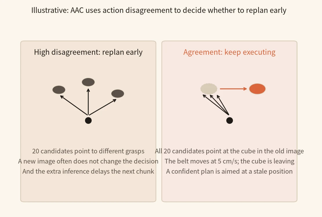
The best s also depends on how long the model was trained. With the same 20-step prediction, the model trained for 1,000 steps works best at s = 5, and the model trained for 5,000 steps works best at s = 15. The authors also tried AAC (adaptive action chunking), which lets the model choose s itself: it samples 20 candidate chunks at once, checks how much they disagree, and replans early when they disagree a lot. AAC never beat the best fixed s and failed on the stationary and fast belts. The authors' explanation is that disagreement is often high because the scene is unfamiliar or several actions are equally fine, and in those cases one more image does not change the decision; when the model is confident, the object may be just about to be carried away. Hoot says
AAC samples 20 candidate action chunks at once, checks how much they disagree, and replans early when they disagree a lot. Below we walk two moments with the red cube on the conveyor. The belt speed of 5 cm/s is from the paper; whether the candidates agree in each moment is illustrative, to follow the paper's explanation, not an experimental result.
Sample 20 candidates → measure disagreement → high disagreement that a new image will not resolve / agreement that keeps executing from a stale image → replans at the wrong moments
- AAC → 20 candidate chunksAAC samples 20 candidate chunks in parallel and uses their disagreement (entropy) to decide how long to keep the current chunk. When disagreement is high, it ends the chunk early and replans from a new image; when disagreement is low, it keeps executing the current chunk for longer.N = 20 candidates
- high disagreement → replan earlyIllustrative first moment: the 20 candidates point to several equally fine grasps, so disagreement is high and AAC replans early. But the scene is unfamiliar, or several actions are equally fine, so one more image does not change the decision, and sampling 20 candidates also delays the next chunk.
- agreement → keep executing from the old imageIllustrative second moment: all 20 candidates point at where the cube is in the image, so the model is confident and disagreement is low. AAC keeps the current chunk going longer and does not look at a new image early.
- conveyor → cube positionThe belt is still carrying the cube away at 5 centimetres per second. The more confident AAC is, the longer it tends to keep the old plan, and the farther the cube moves from the position all 20 candidates aimed at.belt speed = 5 cm/s
- disagreement as the trigger → when it replansSo AAC replans when a new image will not help, and does not replan when the object is about to be carried away but the model is confident. In the paper it never beat the best fixed s, and it failed on the stationary and fast belts.
Source
Main text: AAC never beats the best fixed horizon… Entropy is the wrong trigger here… AAC therefore replans at the wrong moments; Appendix B.2: N=20 candidate chunks. Belt speed 5 cm/s is from the paper's fast conveyor setting. The two moments are an illustrative contrast, not experimental results.Change the model, or change how it is executed
The remaining two methods change the model itself. PUMA feeds the model optical flow from past frames (which way each pixel is moving), computed in both training and inference; during training it also has the model predict the target object's upcoming features, a prediction branch that is not used at inference. It does better than π0.5 on the conveyor but worse on the rolling-can task. Asynchronous execution matters a lot for it: run synchronously, it fails at short s just like the baseline; run asynchronously, it reaches 60% to 70% at every s tested.
DSRL is a reinforcement learning method. It does not change the VLA's parameters. It only trains a small policy that picks the noise input the VLA uses when generating actions. After training on the hardest conveyor condition, success rises from 0 to 60%, and on DOM from 32% to 47%. But it can only pick out actions the VLA already knows how to produce, and the gain disappears when the noise is turned up.
Averaged over the nine conveyor conditions, DSRL lifts the model trained for 1,000 steps to 64% to 69%, and some conditions get worse. The same model with no training at all, with s set to 5, reaches 71%. In the authors' words, changing how the policy is executed was worth as much as training it.
What this means for people building robot policies
When you evaluate whether a VLA works on dynamic tasks, treat the execution setup as an experimental variable and report it together with the model.
Before comparing two models, fix one execution setup: how many seconds to predict, how many steps to execute, synchronous or asynchronous, and what action rate. Otherwise a 10-point gap between two models may just mean one of them happened to get a good s. The paper suggests reporting three quantities next to the success rate: observation age, how soon a new action becomes available, and how much the arm jumps between old and new chunks.
If you want an existing model to react faster in dynamic scenes, start with changes that cost no training: switch to asynchronous inference, add a step that aligns new and old chunks, raise the action rate, and sweep a few values of s. After trying these, consider reinforcement learning fine-tuning or adding motion information.
Limitations
All conclusions are based on π0.5. The authors ported FASTER, DynamicVLA, ABPolicy, and the other methods to π0.5, taking only part of each original mechanism, rather than reproducing the full original systems.
There are few tasks. Each real-robot setting has only 15 to 20 trials, and in the rolling-can and moving-cup tasks the objects are moved by hand, so the trajectories differ from trial to trial; the authors themselves caution against over-reading small differences. Not every method was tested at every s; ABPolicy was tested only at s = 9.
How did this read for you?
Hoot made a note. Thanks for the feedback.

One tap, no sign-in; tap again to undo. Only anonymous counts are kept, never who you are.
Related papersMore from Paper Daily
 Embodied · 2026-11-16Scaling VLA Serving Under Robotic Execution ConstraintsThe authors' company already has hundreds of VLA-driven robots working in real environments, and robots must share GPUs to keep inference costs down. Robots keep executing old actions while waiting for new ones. So among requests of the same size, some robots are about to run out and need a reply now, while others can wait. Admitting one more request on the GPU also slows the requests already run…
 Embodied · 2026-10-27Coupling Execution Horizon and Sampling Depth in Flow-Matching VLA PoliciesIn flow-matching vision-language-action models, solver steps and execution horizon turn out to be coupled, and the best setting can reverse. These models start from random noise and use a numerical solver to push it step by step into a smooth action chunk. Deployment usually tunes the two separately: the horizon amortizes inference latency, while solver steps stay high for accuracy. Under frequen…
 Embodied · 2026-11-04ReGATE: Recurrent Gated Visual Fusion for Reactive Humanoid-Object InteractionWhen a humanoid robot reaches for a box, the box blocks its head depth camera as soon as the hands get close, yet the controller still has to finish the whole sequence of picking up, carrying and putting down. This paper lets the robot act mainly through the joint-state pathway and treats the depth image only as a correction scaled by learned gates, designed to let less of it in when the image is…
Discussion
Add experiment details, reproduction notes or a different take. Requires a GitHub sign-in.
Loading the discussion…