Contents · 8 sections
1Distance alone treats the two films as the same2Three quantities: gap, surrounding knowledge, the jump you are used to3Five axioms collapse into one formula4Walking through it: one film, three viewers5Survey: does the computed curiosity match what people report?6Offline and online: how much does adding it change7What this means for people building recommenders8LimitationsSHARE

Two films equally far from your taste: why does only one make you want to click? Measuring curiosity for recommendersYour home feed shows two films you have not seen. By the recommender's distance, both sit equally far from your taste. The difference: the first is surrounded by many similar films you have watched, while you have watched nothing at all near the second.
You will probably be curious about the first. You know roughly how such films go, and you want to see what this one does differently. The second likely leaves you cold, because you cannot even tell what you are missing. Yet the common "unexpectedness" family of metrics looks only at distance and gives both films the same score.
This working paper by Li and Tuzhilin computes a score for "how much curiosity this item evokes in this person right now" and puts it into ranking. Three kinds of existing methods come closest. Unexpectedness scores an item by how far it sits from what the user expects, with one fixed preferred distance per user. Variety-seeking treats "likes trying new things" as a stable user trait that scales unexpectedness up or down. Wundt-curve methods assume too little stimulus bores and too much repels, and estimate one fixed optimal stimulus per user. None of them asks how much the user already knows around this particular item. Starting from the information-gap theory of curiosity in psychology, the authors write five axioms, add four shape conditions, and derive a curiosity formula with a single free parameter. In a 283-person survey, with the designed gap levels, this score matches self-reported curiosity better than the alternatives; more importantly, the most curiosity-evoking gap moves across people the way the formula predicts. Added to an existing relevance score, it beats those metrics and diversity re-rankers on three offline datasets, and in a one-month A/B test on a large Asian video platform it raised click-through by 2.75 percentage points; the platform then deployed it.
How far away the most intriguing item should be depends on how much you have seen around it and how big a jump you are used to lately; the online evidence comes from one video platform and one experiment using a simplified formula.
Distance alone treats the two films as the same
Unexpectedness, variety-seeking and the Wundt curve share one trait: the score is driven by the item's distance from the user, and the preferred distance is a single fixed value per user.
The two films in the opening are their blind spot. Same distance, same preferred distance, same score. But curiosity needs some prior knowledge. Information-gap theory (Loewenstein 1994) says you must know part of something before you notice that part is missing; someone who knows nothing feels only indifference.
The theory adds that the gap is relative. A gap of the same size may be too large for someone who has been watching familiar content lately, and just right for someone who has been switching genres.
So the score has to look at three things at once.
Three quantities: gap, surrounding knowledge, the jump you are used to
The first is the information gap g: the Euclidean distance between the item vector and the user state. Item vectors come from an AutoEncoder over features such as title, genre and director. The user state is the hidden state of a GRU after reading the user's history in order, trained so that this distance predicts whether the user clicks. A larger g means the item is less familiar to this user.
The second is the surrounding context f, between 0 and 1. Each item the user has watched gets a weight by how close it is to the candidate, closer meaning larger; the weights are summed and squashed into 0 to 1. So f is near 0 when the user has watched nothing nearby, and approaches 1 as more and closer items pile up. History far from the candidate adds almost nothing.
The third is the reference gap τ: the average of the gaps the user has recently experienced, with recent ones weighted more. Someone who spent last week on familiar sitcoms met only small gaps, so τ is small. Once he starts trying new genres this week, τ grows. τ can be updated recursively after each item, without rescanning the whole history.
Five axioms collapse into one formula
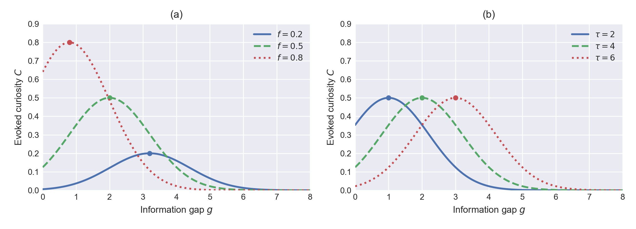
The authors split information-gap theory into five axioms. Curiosity depends only on g, f and τ. With no surrounding knowledge (f = 0) or an infinitely large gap, curiosity is 0. The larger f, the smaller the most curiosity-evoking gap: a film scholar is drawn to fine differences in how two directors handle the same scene, while a newcomer needs a much bigger gap to feel anything is worth knowing. The larger τ, the larger that gap. τ is a recency-weighted average of past gaps.
The axioms only say that curiosity is 0 at both ends, has a highest point in between, and which way that point moves; they do not fix the shape of the curve, and infinitely many functions satisfy them. A recommender needs one formula it can compute. The authors add four shape conditions, for example: the peak sits at τ when f is near 0 and at 0 when f = 1, moving evenly with f in between; the peak height is 0 at f = 0 and 1 at f = 1, also changing evenly. They prove that exactly one formula meets these conditions: Hoot says
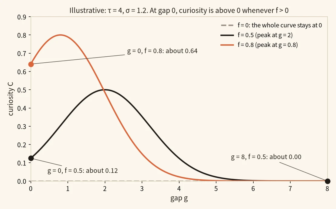
Keep the body's τ = 4 and σ = 1.2; the formula is C = f × exp(−(g − τ(1 − f))² ÷ 2σ²). Below we push the gap g to both extremes; the numbers are illustrative.
f = 0 → the whole curve is 0; f > 0 → gap 0 still scores → only a huge gap brings it to 0
- surrounding knowledge f = 0 → the whole curvef is the multiplier in front and also the peak height. At f = 0, curiosity is 0 whatever the gap.0 × exp(…) = 0
- gap g = 0 → Ann's curiosityAnn has f = 0.5, so her peak is at τ(1 − f) = 2. A candidate with gap 0 sits 2 away from the peak and scores about 0.12, above 0.0.5 × exp(−2² ÷ 2.88) ≈ 0.12
- more knowledge → higher at gap 0Ben has f = 0.8, so his peak moves to 0.8, only 0.8 from gap 0. A nearly identical film scores about 0.64 for him, like a film scholar drawn to fine differences.0.8 × exp(−0.8² ÷ 2.88) ≈ 0.64
- huge gap → zeroPush Ann's gap to 8, 6 away from her peak, and the exponential is nearly 0. This is the other end the axioms mean by "0 when the gap is infinite".0.5 × exp(−6² ÷ 2.88) ≈ 0.00
So "0 at both ends" means two conditions: no surrounding knowledge at all, or an infinite gap. At gap 0, curiosity is above 0 whenever f is above 0.
Source
paper section 3, the five axioms and the curiosity formula; τ = 4 and σ = 1.2 from paper Figure 3.3; f = 0.5 and 0.8 are Ann's and Ben's values in the body walkthrough; gaps g = 0 and 8 are illustrativecuriosity C = f × exp(−(g − τ(1 − f))² ÷ 2σ²)
In words: curiosity rises and then falls with the gap, peaks at g* = τ(1 − f), and the peak height is f. σ only sets the width of the curve and is the only parameter to tune. The appendix shows that replacing one shape condition gives a different family of formulas, while the qualitative predictions of the five axioms stay the same.
Walking through it: one film, three viewers
We use the parameters of the paper's Figure 3.3: σ = 1.2, τ = 4. The simplified way of computing f and τ comes from the online experiment in Appendix D; the viewing histories are illustrative.
Step 1, surrounding context f. The online version takes the user's 10 most recent films and counts how many lie within distance 0.1 of the candidate. Ann has 5, so f = 5 ÷ 10 = 0.5, meaning half of her recent films sit next to this candidate.
Step 2, reference gap τ. The online version averages the gaps these 10 films had with Ann when she watched them. Ann's recent average gap is 4, so τ = 4.
Step 3, the peak. g* = τ × (1 − f) = 4 × 0.5 = 2. For Ann, films at gap 2 are the most intriguing.
Step 4, the candidate's score. The candidate's gap to Ann is exactly 2, right on the peak, so C = 0.5 × exp(0) = 0.5.
Step 5, two more viewers, same gap and same τ. Ben is an expert: 8 of his last 10 films sit next to the candidate, f = 0.8, so the peak moves to 4 × 0.2 = 0.8. Gap 2 is 1.2 past the peak, exactly one σ, so the curve drops to about 0.61 of its height: C ≈ 0.8 × 0.61 ≈ 0.49.
Cam is nearly a newcomer: only 2 nearby films, f = 0.2, so the peak sits at 4 × 0.8 = 3.2. Gap 2 is 1.2 short of the peak, again one σ, so C ≈ 0.2 × 0.61 ≈ 0.12.
The same film scores 0.5, 0.49 and 0.12. A distance-only metric sees the same distance for all three, and can only differ through each person's fixed preferred distance. Here the difference comes from f: Cam knows almost nothing in this area, so his whole curve is pressed down. Ben knows the area too well; finer differences intrigue him, and a gap of 2 is too big for him.
Once scored, ranking uses V = (1 − α) × relevance + α × w × C, with both terms standardized first. w is how responsive this user is to curiosity: regress his past engagement on C, holding relevance fixed, and take the coefficient on C, floored at 0. α is a platform-level weight. Relevance can come from any existing model, DIN or MF alike, without changing it.
Survey: does the computed curiosity match what people report?
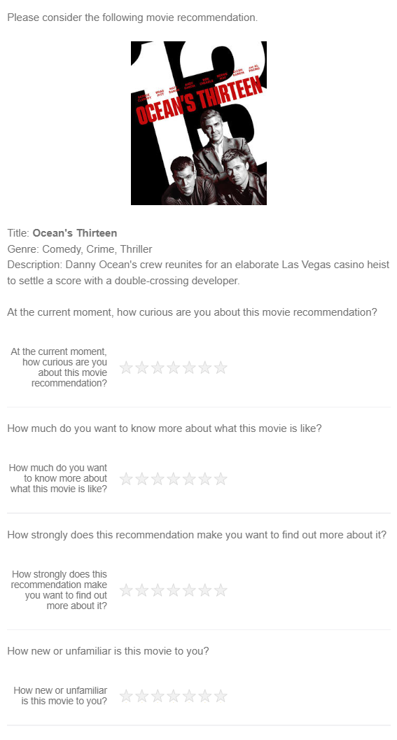
The authors built a survey with films from MovieLens. Each participant saw 15 recommendation cards in turn, each with poster, title, genre and a short description, then answered several 1-to-7-star questions; three of them asked about curiosity and were averaged into a curiosity score. Films were chosen to fill a grid of 6 gap levels × 2 context levels, plus a few films with almost no surrounding context, so every participant saw the whole curve. 300 people answered, 283 passed the attention check, giving 4,245 ratings.
Key results:
| Test | Result |
|---|---|
| Correlation with reported curiosity | 0.636 with designed gaps, 0.598 with model-computed gaps; unexpectedness 0.603, variety-seeking 0.589, Wundt 0.611 |
| After controlling for perceived novelty and unexpectedness | C adds 0.245 to R²; novelty and unexpectedness add at most 0.027 |
| Films with almost no surrounding context | 1.41 stars on average, almost no curiosity |
| Film most similar to one's favourite | 1.48 stars, also almost no curiosity |
| Most curiosity-evoking gap | 2.80 at low context, 1.87 at high context |
| Three reference-gap groups (low context) | peaks at 1.72, 2.70, 3.73 |
(Numbers from the paper's Table 5.2 and Section 5.2)
The first row needs care. With designed gaps, C beats all three older metrics; with model-computed gaps, 0.598 is already below Wundt's 0.611 and unexpectedness's 0.603. On correlation alone, the advantage is not robust.
The later rows carry more weight. After controlling for novelty and unexpectedness, C still explains about 24% extra variance in reported curiosity, while those two add almost nothing. Films at both ends barely intrigue anyone and the middle is highest, whereas novelty keeps rising with the gap, so novelty alone cannot draw this shape. The peak also moves in the predicted direction: more knowledge, nearer peak; bigger recent jumps, farther peak. Older metrics have one fixed preferred distance per person and cannot explain this movement.
Offline and online: how much does adding it change
Offline experiments use Yelp, MovieLens and Alibaba-Youku, with DIN and MF as relevance models. For fairness all methods share the same AutoEncoder item vectors. Unexpectedness and the other older metrics are combined with relevance through the same formula as C; the two diversity re-rankers, MMR and DPP (determinantal point processes), use their own re-ranking trade-off parameters. Every method is tuned on the validation set with the same budget.
| HR@10 on DIN | Yelp | MovieLens | Alibaba-Youku |
|---|---|---|---|
| DIN only | 0.409 | 0.422 | 0.113 |
| Best older metric | 0.491 | 0.477 | 0.163 |
| Plus curiosity C | 0.512 | 0.495 | 0.216 |
| C with f and τ both set to sample medians | 0.473 | 0.451 | 0.193 |
(Numbers from the paper's Tables 6.3 and 6.4)
According to Table 6.3, adding C gives the highest hit rate, NDCG, diversity and novelty of all methods on all three datasets, and the same holds with MF; the table above only excerpts HR@10 on DIN. The last row is an ablation: fixing f and τ at everyone's median leaves C depending on the gap alone, with the peak at the same place for every user. This version already falls below the best older metric on Yelp and MovieLens. So much of C's lead over older metrics comes from "the peak moves with the person"; "rise then fall" alone is not enough. Dropping only the recency weighting of τ costs the least: Yelp goes from 0.512 to 0.489.
The curiosity weight α also has to be tuned per platform. MovieLens averages 151 records per user and its hit rate peaks around α = 0.4; Yelp and Youku have only 34 and 40 per user and do best with α near 1.
The online experiment ran for one month in 2021 on an Asian video platform with over 500 million monthly active users. 516,201 users were randomly split: the control group used the production DIN, and the treatment group added the curiosity term to the same relevance score, over 26,959,538 recommendation records. Because of latency limits, the treatment used the simplified computation from the walkthrough: f counts how many of the last 10 films lie close enough, τ averages the gaps of the last 10. Click-through rose 2.75 percentage points, completed views 1.97 points, and watch time 0.71 minutes per recommendation, all significant at 1%. Only the absolute change is reported, with no control-group base rate, so the relative lift cannot be computed.
Where the effect is largest also fits the theory. Each standard deviation of deeper history adds 0.87 points of click-through; each standard deviation of more recent activity adds 1.19 points. The interaction for users over 60 is −13.84 points, and for big-city users −9.15 points. Both are relative to users with no age or city given, which shows these groups gain clearly less than the reference group; only the interaction terms are reported, not the reference group's own effect, so whether their net effect is negative cannot be computed.
What this means for people building recommenders
Before adding exploration, measure how much the user has already seen around a candidate, then decide how far away is right for him.
The item vectors and sequential user states this score needs already exist in most recommenders. The simplified online version needs only the last 10 history items: count how many sit close to the candidate and average their 10 gaps, which is cheap. To try it, compute f, τ and C for each impression in offline logs and check whether clicks peak where g is near τ(1 − f) before putting it into ranking.
The second point is per-user weighting. The paper's subgroup results show younger, premium and recently active users gain most, while users over 60 and in big cities gain clearly less. The authors suggest raising the curiosity weight for the former and lowering it for users who prefer familiar content.
Limitations
The online experiment was run in 2021 on one platform with the simplified formula, and the online values of σ and α are not given. Nor is the control group's click-through base rate, so only percentage-point changes are available.
The survey used MovieLens films and self-reported curiosity, a different setting from scrolling videos. With model-computed gaps, C correlates 0.598 with self-reports, below the Wundt curve.
Only σ is fitted from data; the peak location τ(1 − f) and height f come from the shape conditions the authors chose. Other shape conditions would give other formulas.
The model cannot see what users watched off the platform, and it assumes nothing watched is forgotten.
How did this read for you?
Hoot made a note. Thanks for the feedback.

One tap, no sign-in; tap again to undo. Only anonymous counts are kept, never who you are.
Discussion
Add experiment details, reproduction notes or a different take. Requires a GitHub sign-in.
Loading the discussion…