Contents · 7 sections
1One small experiment can kill a useful change2Good and bad changes produce loss curves of the same shape3How five small-scale points become a probability4Five small scales add up to about 55% of one full run5On HSTU most calls are right, with some false passes and misses6Back to genre: where the method breaks7Small-scale runs in exchange for a probabilitySHARE

This Meta paper argues that whether a recommendation-model change deserves full-scale rollout should not be decided by who wins one small-scale run, but by the probability that the loss curve traced across five small scales, extrapolated to full scale, beats the baseline by more than a threshold (1% on HSTU).
One small experiment can kill a useful change
Recommendation teams improve a model one candidate change at a time: a new attention structure, a different optimizer, a new input feature. The standard way to confirm that a change helps is a full-scale A/B test: add the change to the production model, retrain from scratch with the full model on the full data, and compare against the control. In industry there can be hundreds of candidate changes, and retraining at full scale for each one is more compute than anyone can afford.
This article follows one running example: adding movie genre to the training prompt of an LLM-based recommender. Illustration: the prompt used to say "Watched: Toy Story (rated 5)", and with the change it says "Watched: Toy Story | Animation/Comedy (rated 5)". Genre makes the prompt longer and inference slower, so it is only worth adding if the gain is clear.
The usual way to save compute is to run one small-scale experiment first: shrink the model, use part of the data, and drop the change if it shows no gain. The paper's motivating example shows exactly how this goes wrong. On MovieLens-20M, the treatment with genre has lower HR@10 than the control at small scale, yet is clearly better at full scale. Judging by the small run alone, this useful change would have been dropped.
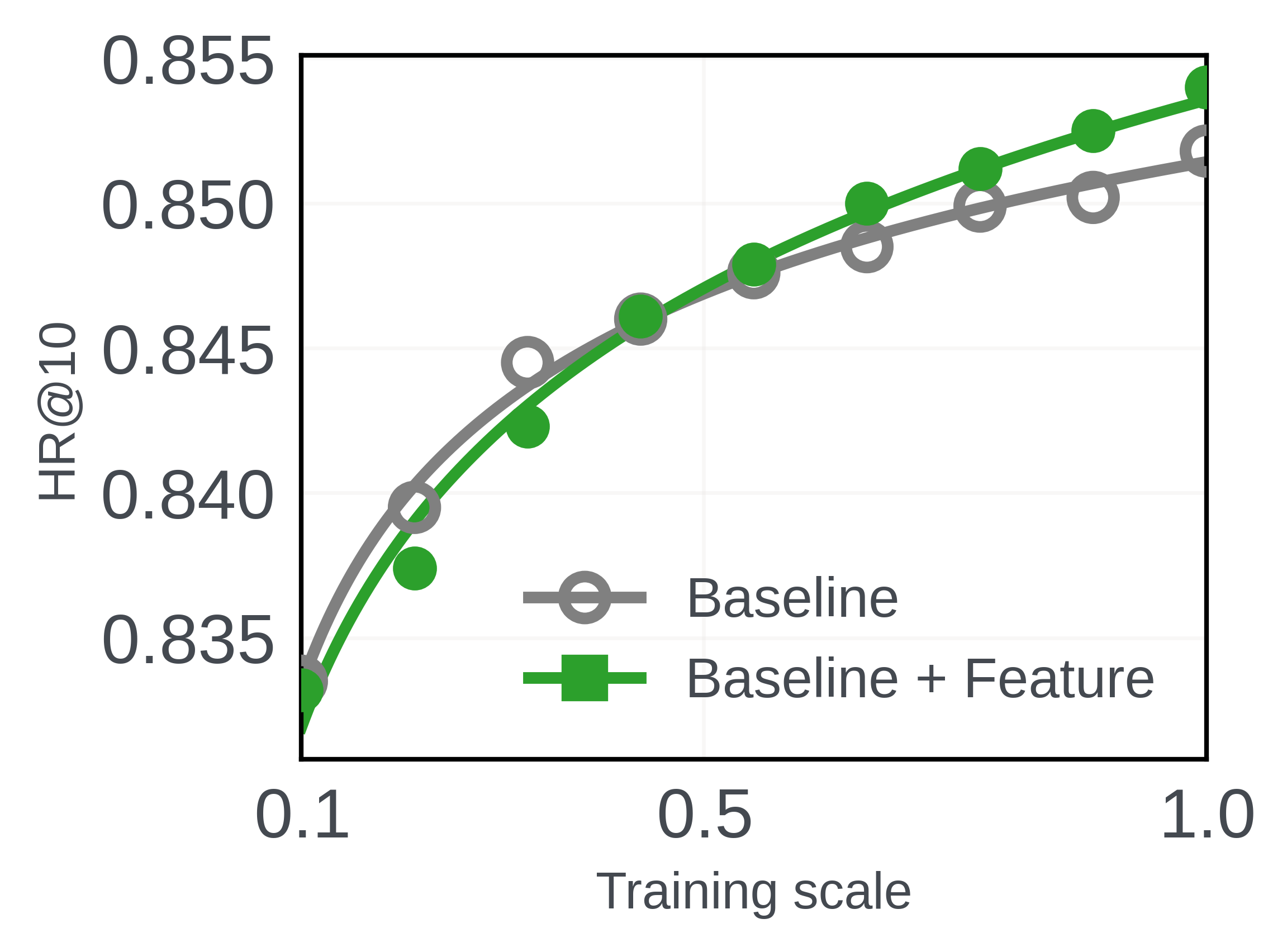
Picking a single, somewhat larger scale does not fix this. Across many changes, the authors see that different categories of changes flip direction at different small scales, so there is no way to know in advance which scale gives a trustworthy signal.
Good and bad changes produce loss curves of the same shape
The two curves in the previous section's figure cross, but each one is very regular on its own. The authors fit a power law Loss = θ1·N^θ2·D^θ3 (N is the parameter count, D the amount of training data), and both the baseline and the treatment reach R² above 0.99, just with different coefficients.
The authors call this feature-invariant scaling: whether a change helps or hurts, the model's validation loss as a function of scale stays within the same family of power laws. Same family here means the same functional form, not overlapping curves. Hoot says

Illustrative, not paper results: x is training scale s, merging model and data scaling into one axis as in Figure 3; a and c are illustrative.
Source
functional form: paper §3, §4 (Figure 3, Table 1); θ1, θ2, θ3 notation: §5.2; single training-scale axis: §5.3; a, c illustrativeWukong is a recommendation model for click-through-rate prediction on Criteo; the authors add dropout to it, switch its optimizer to SGD, or add an attention layer (Figure 3). Dropout helps and SGD hurts, yet the three curves still fit with R² of 0.9953, 0.9923, and 0.9876 (Table 1).
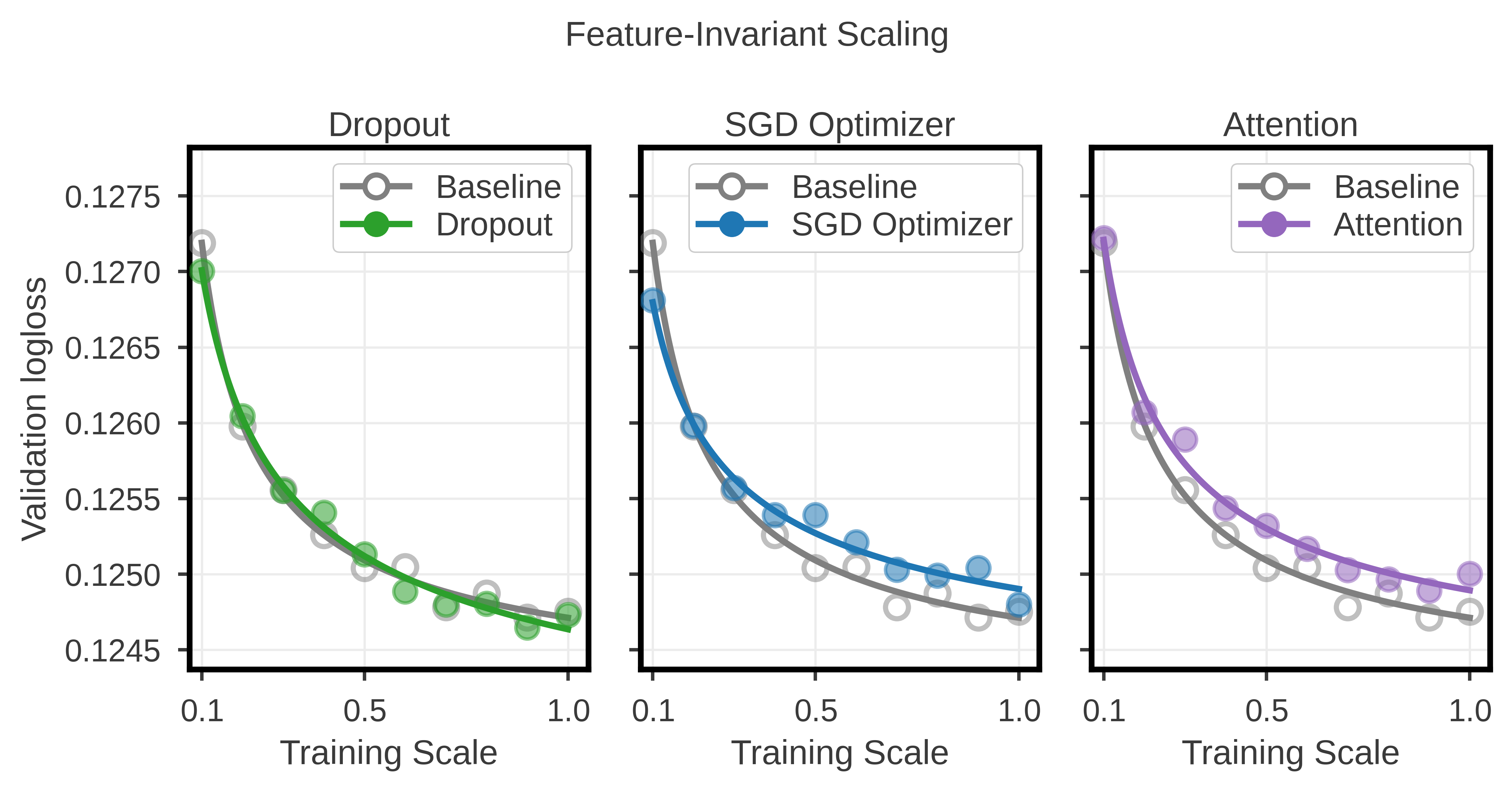
No panel's curve coincides with the baseline, and the SGD curve even crosses it, yet all share one shape: a steep drop that then flattens.
Across more than 40 changes on three model families (Wukong, HSTU, and LLM-based recommenders), the power-law fits have R² between 0.9743 and 0.9989 (Table 2). This means the functional form can be fixed in advance, leaving each change only its own power-law coefficients to estimate. The authors describe this as the first work to point this out.
How five small-scale points become a probability
The method assumes the baseline's full-scale validation loss is already known, which is normal in industry: the production model has been trained anyway. Only the treatment is trained, in four steps:
| Step | Input | Operation | Output |
|---|---|---|---|
| 1 | One candidate change | Train once at each of scales 0.1, 0.2, 0.3, 0.4, 0.5 | Five (scale, validation loss) pairs |
| 2 | The five observations | Fit one power-law curve along the scaling path actually used (scale 0.1, 0.2, ...) | One power-law curve and residual noise σ |
| 3 | The fitted model | Extrapolate to full scale 1.0 | A Student-t distribution over full-scale log loss |
| 4 | That distribution | Compute its mass below "baseline loss × 0.99" | A probability; the change passes only above 90% |
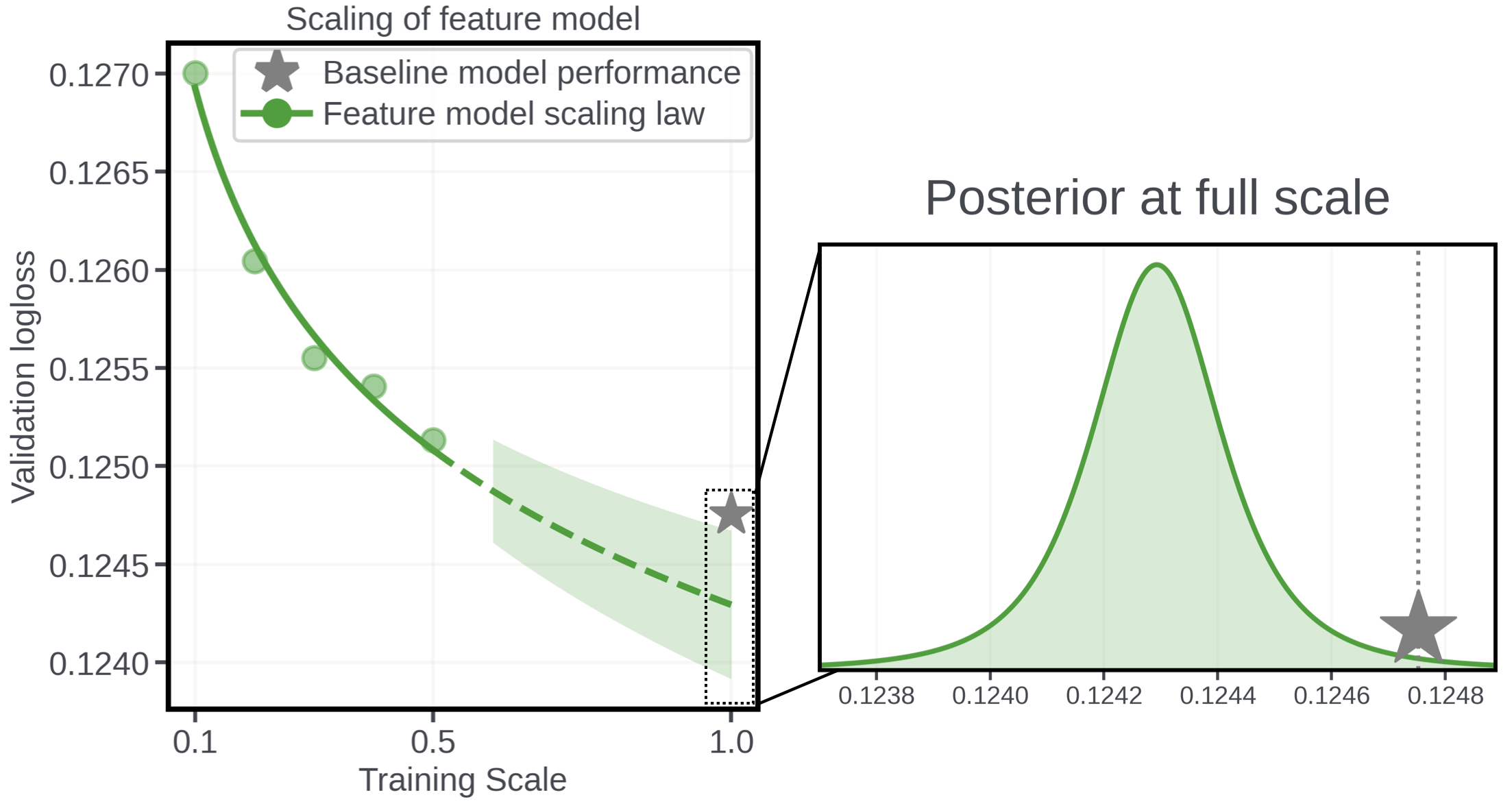
Step 3 produces a distribution rather than a point. The noise σ is also estimated from the same small-scale points, so the method uses a Student-t distribution, whose tails are heavier than a normal's, and heavier the fewer points there are. Its center is the fitted curve's log loss extrapolated to full scale, and its width is σ times a factor set by where the small-scale points sit and how far full scale lies from them, growing the farther the extrapolation goes. It describes how uncertain the estimate of full-scale log loss is given only these small-scale points, which the paper calls the posterior distribution conditioned on the small-scale observations.
Step 4 sets the bar at "more than 1% better"; being only slightly better than the baseline does not count. Marginal gains do not justify deployment, especially for a change like genre that slows inference. The authors cite the HSTU paper: in industrial settings, a 0.1% reduction in loss typically brings more than a 0.5% increase in topline metrics across billions of users.
Back to the genre example, here is a set of illustrative numbers to show what the intermediate output looks like. Suppose the curve fitted to the five points amounts to "each doubling of scale multiplies loss by 0.98", and the loss at scale 0.5 is 0.1250. Going from 0.5 to 1.0 is exactly one doubling, so the center of the full-scale prediction is 0.1250×0.98 = 0.1225.
Set the baseline's full-scale loss to 0.1226. Genre is an LLM-recommender change, so the bar uses the 0.05% margin: 0.1226×0.9995 ≈ 0.12254. Written out, the output of steps 3 and 4 is a line like this (illustrative):
{center: 0.1225, 90% interval: [0.1219, 0.1231], bar: 0.12254, probability below bar: 0.57}The center is already below the bar, so a point estimate alone would pass the change; but the interval straddles the bar, and 57% is below 90%, so the rule does not pass it. This shows what the rule guards against: noise in five points happening to pull the curve down a little.
Five small scales add up to about 55% of one full run
When the model and the data are shrunk together, scale 0.5 means both are halved, which costs about a quarter of a full run. The five points cost about 0.01, 0.04, 0.09, 0.16, and 0.25, which sum to 0.55. So each change spends a bit over half of one full run and gets back a decision with a confidence level attached.
The authors point to a further benefit: experiment machines often cannot hold the full-scale model in memory, in which case a full-scale A/B test cannot run at all, and shrinking the model is the only option.
This accounting holds only when model and data shrink together. The paper's LLM experiments keep the model fixed and shrink only the fine-tuning data, so each point's cost falls only with the data size, and the 0.55 figure no longer applies.
On HSTU most calls are right, with some false passes and misses
The main experiment uses HSTU for next-movie prediction on MovieLens-20M. Full scale is HSTU-large (embedding dimension 256, 16 blocks, 8 heads); scale 0.1 shrinks it to 26 dimensions, 2 blocks, and 1 head. The three dimensions shrink together so that the small models keep a shape similar to the full one. Each change is trained at 0.1–0.5 and decided by the rule "probability of being more than 1% better > 90%".
The table below picks a few rows; first, what each change does. Wider Head 48 raises the per-head Q/K/V dimension from 32 to 48. Attn Res lets each block learn a weighted read of the outputs of all preceding blocks. Extra Block adds one more HSTU block. Time Gap Bias adds a learned decay to attention based on the elapsed time between interactions. Softmax replaces HSTU's pointwise SiLU attention with softmax attention. Weight Decay 0.1 changes AdamW weight decay from 0 to 0.1. HSTU's attention also has an RAB term (relative attention bias, a bias based on the distance and time difference between two positions), and No Temporal RAB removes its time component.
| Change | Probability, 0.1–0.4 | Probability, 0.1–0.5 | Actual full-scale loss change | Under the 90% rule |
|---|---|---|---|---|
| Wider Head 48 | 98.7% | 98.7% | −7.3% | Passed, correct |
| Attn Res | 64.6% | 90.8% | −1.5% | Passed, correct |
| Extra Block | 67.1% | 72.9% | −1.3% | Missed a good change |
| Time Gap Bias | 78.8% | 79.9% | −0.8% | Not passed, below 1% |
| Softmax | 92.2% | 91.2% | +1.0% | Wrongly passed a bad change |
| Weight Decay 0.1 | 17.7% | 3.9% | +16.6% | Blocked |
| No Temporal RAB | 4.6% | 1.1% | +8.7% | Blocked |
This shows that large gains and large regressions are separated cleanly: the change that is 7.3% better at full scale gets 98.7%, and the one that is 16.6% worse gets 3.9%. The errors cluster around changes whose full-scale effect is near 1%: Softmax is actually 1.0% worse but gets 91.2%, while Extra Block is actually 1.3% better but gets only 72.9%. The Attn Res row also shows that more points help: 64.6% with four points, crossing the bar only once 0.5 is added.
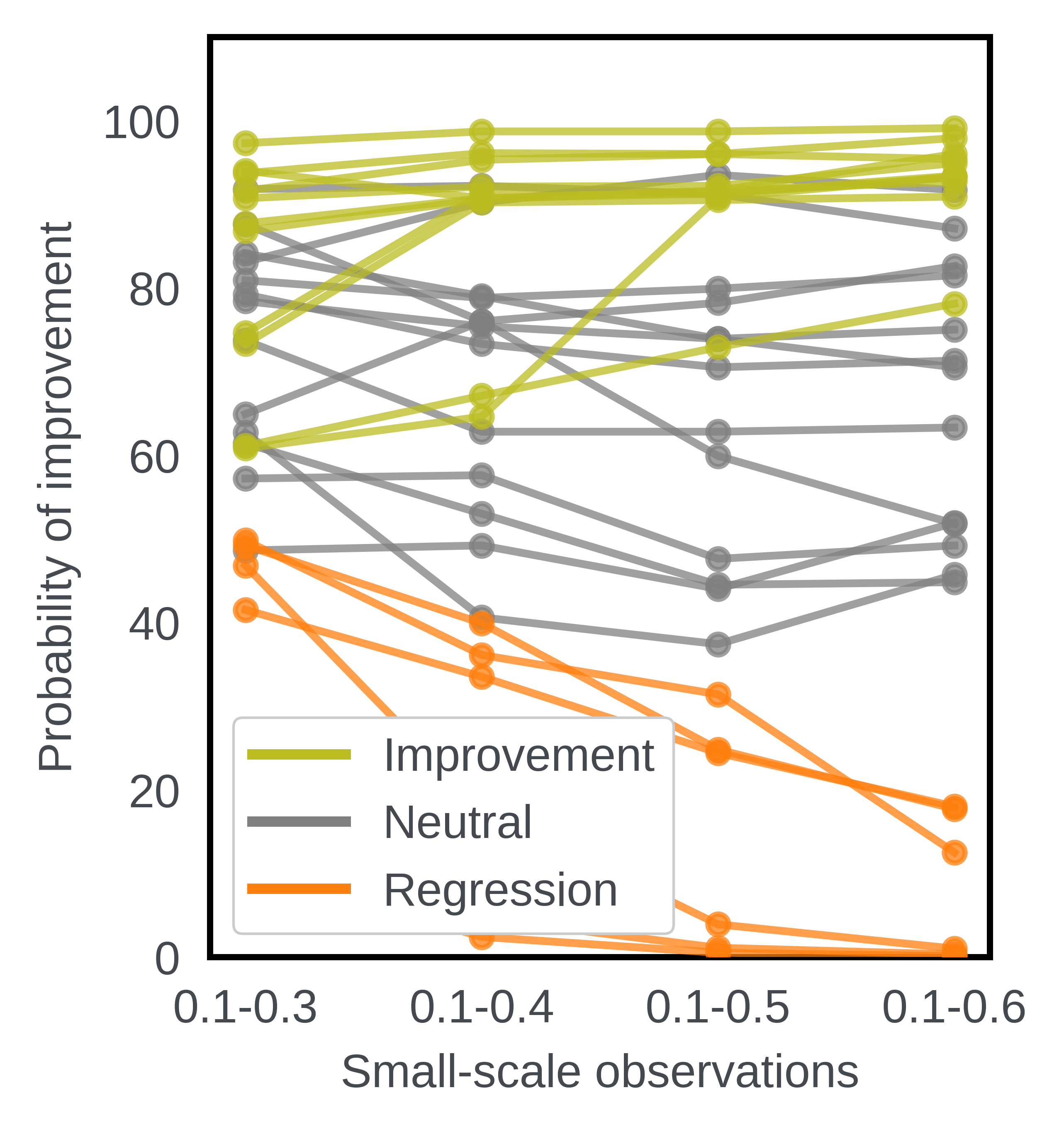
In Figure 6, as points are added, the probability for changes that actually help mostly climbs toward 100%, and for harmful ones falls toward 0. The authors also report that the out-of-sample prediction error for full-scale loss shrinks as more points are added.
The paper also lists several examples of beneficial changes: put back into HSTU-large, they move HR@10 on MovieLens-20M from the baseline's 0.3567 to 0.3581–0.3603. The highest is Time Gap Bias (+1.01%), followed by Dropout 0.1 (+0.64%). My reading: Time Gap Bias lowers loss by only 0.8%, below the 1% bar, yet gains the most in HR@10, which means the loss bar and the final ranking metric are not fully aligned.
Back to genre: where the method breaks
Changes on Wukong and the LLM recommender all have effects below 1%, so the authors use a 0.05% bar for them. In the running example, genre on Llama-3.1-8B lowers full-scale loss by 0.5%, yet the five points at 0.1–0.5 give a probability of only 60.2%, reaching 91.1% only when 0.6 is added. So in the genre case it takes a sixth point to cross the bar.
Wukong's Attention swings the same way: 92.2% at 0.1–0.4, dropping to 0.0% once 0.5 is added, and it is actually 0.1% worse at full scale. This shows that with too few points, the conclusion can flip when a single point is added.
The same change on a different base model can also go the other way: genre makes Llama better but Qwen worse. In both cases the power law still holds, and the method still predicts the direction correctly.
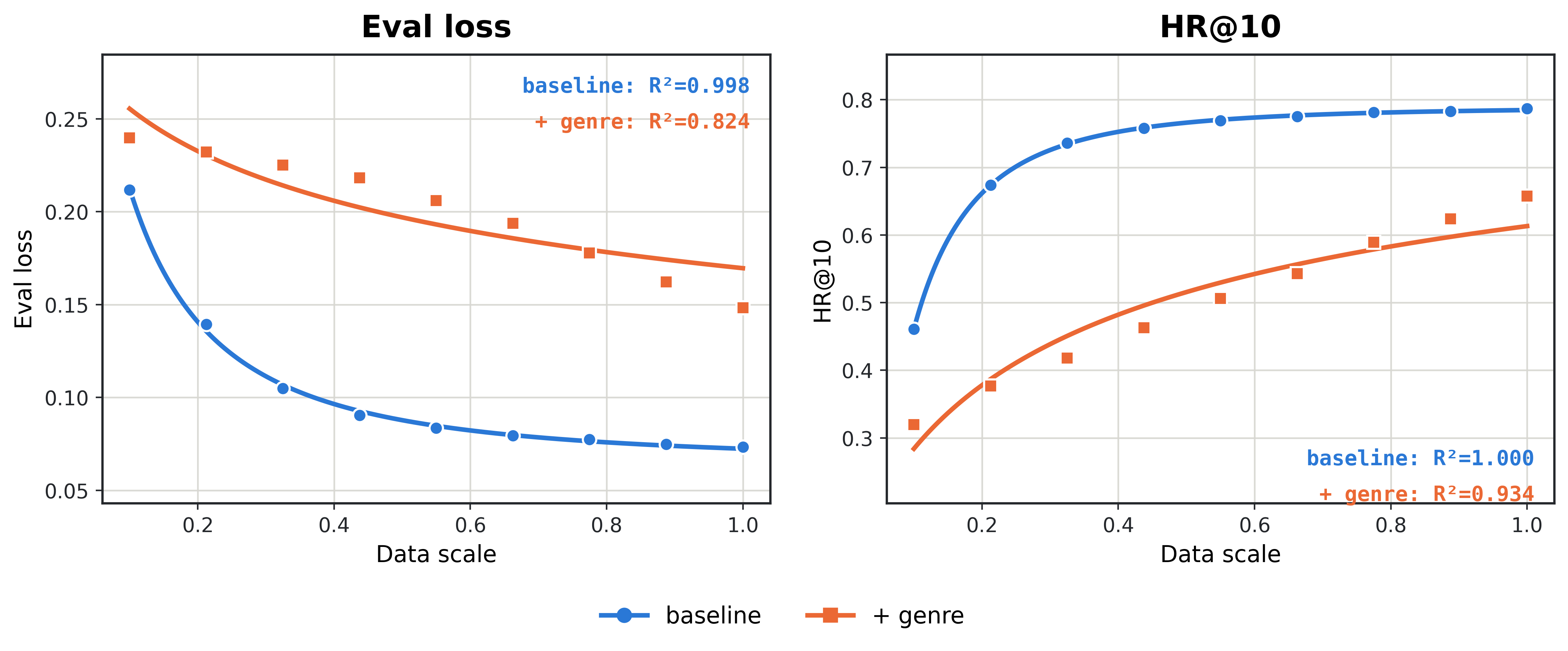
What actually breaks the method is the power law itself failing. On Qwen-0.5B with genre added, the loss curve no longer follows a power law, the figure shows an R² of only 0.824, and performance is clearly worse than the baseline. The authors' guess is that genre makes the context about 30% longer and the small model cannot absorb it. In that case the extrapolated probability has no basis; the authors concede such cases would hinder the method but expect them to be uncommon.
Small-scale runs in exchange for a probability
Back to the opening question: whether to add movie genre, a single run at scale 0.1 says "don't". The paper's approach spends a few more small runs, connects the small-scale points into a power law, and asks how confident the extrapolation to full scale is about clearing the bar. For genre itself, at the 0.05% bar the five points give only 60.2%, and it takes a sixth point to pass 90%.
What this method saves is the full-scale retrain, and what it returns is a probability that can be wrong, but wrong in visible places: on HSTU the misjudgments cluster around changes near 1% at full scale, and the method breaks when the curve itself does not look like a power law.
How did this read for you?
Hoot made a note. Thanks for the feedback.

One tap, no sign-in; tap again to undo. Only anonymous counts are kept, never who you are.
Related papersMore from Paper Daily
 Generative · 2026-07-29Realizing Scaling Laws in Recommender Systems: A Foundation-Expert Paradigm for Hyperscale Model DeploymentDeep dive: Realizing Scaling Laws in Recommender Systems: A Foundation-Expert Paradigm for Hyperscale Model Deployment.
 Personalization · 2026-10-20Predictable Scaling: Efficient Model Exploration via Scaling-Law PredictionPredictable Scaling evaluates ranking-model changes with reduced-scale proxies and estimates their full-scale effects using historical learning curves. Training compute falls by 88% and 79% on two industrial ranking models.
 Personalization · 2026-10-28Unified Heterogeneous Feature Interaction via Effective-Rank Scaling for Recommender SystemsMost production ranking models squeeze the user's behavior sequence into one fixed vector before it reaches the feature-interaction module, so later interaction layers can no longer see which clicks or add-to-carts actually happened. Alibaba Taobao's HiRank keeps the behavior sequence alive through every layer of the backbone, and builds the retrieval query over long-term history from the user's…
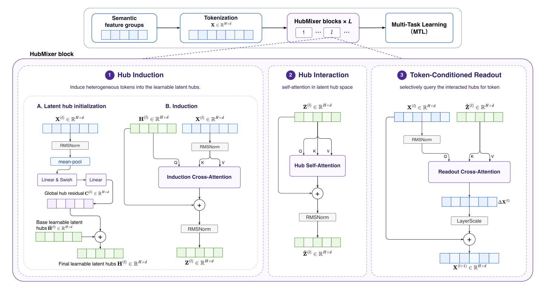 Personalization · 2026-09-01HubMixer: Progressive Latent Hub Mixing for Parameter-Efficient Feature Interaction in RecommendationDeep dive: HubMixer: Progressive Latent Hub Mixing for Parameter-Efficient Feature Interaction in Recommendation.
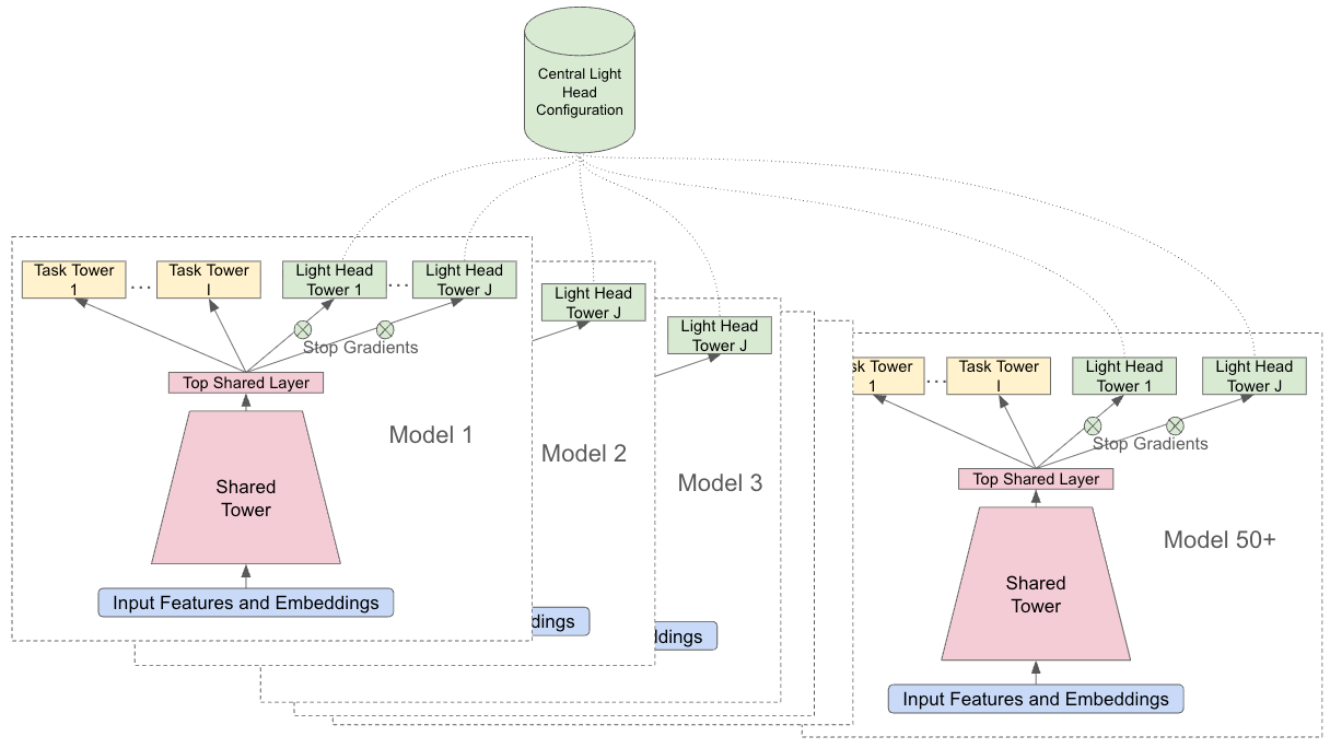 Personalization · 2026-11-03Lightweight Ranking Heads: Accelerating Multi-Task Experimentation in Production Recommender SystemsThe bigger a multi-task ranking model gets, the slower it becomes to add a new prediction target. YouTube's answer keeps the new target out of the main model and makes it a small prediction head on top of the shared layers (the paper calls it a Light Head). It only reads the shared layers' output, sends no gradient down, and is reset at the start of every training run, and every ranking model rea…
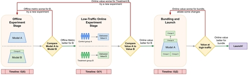 Personalization · 2026-10-24A Framework for Value-Aligned Modeling and Robust ExperimentationIn the Google Discover ads team's model iteration, offline and online results did not line up. The correlation between the change in the conversion model's offline loss and online advertiser value was only 0.1, and many changes that looked better offline failed in the small-traffic A/B stage. This paper weights the offline loss by how much each click is worth to the advertiser, so that a loss dec…
Discussion
Add experiment details, reproduction notes or a different take. Requires a GitHub sign-in.
Loading the discussion…