Contents · 6 sections
1Three requests, one kind of waste2Before drafting, estimate a triangle table from the target model's own state3The reward curve is not concave, so cover it with a concave envelope first4After sorting, put a price on drafting time5Same checkpoint, over 60% less drafting time6Gains concentrate at high load, and there are costsSHARE

ForeSpark shows that under high load, parallel speculative decoding wastes its compute on drafting, not on verification: every request writes all 15 draft tokens, and only 3 to 4 of them get verified. The way to save that compute is to decide how long each request should draft before drafting starts.
Speculative decoding lets a small drafter guess the next few tokens, then has the target model check all of them in one forward pass. The target accepts the run of correct guesses from the start and generates one extra token. The output distribution is exactly the same as token-by-token decoding; each step just emits a few more tokens. Parallel drafters (such as DFlash2 and DSpark) go further: they fill all K positions in a single forward pass, with K=15 by default in this paper, instead of running once per guessed token as EAGLE and MTP do.
Once the batch is large, verification becomes the bottleneck. With 512 requests packed into one step, every extra verified token per request slows the whole batch's step a little, and a wrong guess takes compute away from other requests. Recent systems therefore optimize goodput, the number of accepted tokens per second. DSpark does this with adaptive verification: after drafting, it estimates for each draft position the probability that every guess from position 1 up to this one is correct (called the survival probability below), sorts these probabilities across the whole batch, and verifies only the top ones.
The problem sits before verification. Adaptive verification cuts verification, but every request still drafts all 15 tokens. On Qwen3-14B with 512 concurrent requests, the paper measures that adaptive verification keeps only 3.77 of the 15 drafted tokens per request on average, and drafting takes up to 40% of DSpark's time per token. In other words, about three quarters of the draft tokens never reach verification.
Three requests, one kind of waste
An illustrative batch runs through the whole article. To keep the arithmetic easy, K is 3.
| Request (illustrative) | Content | Expected accepted tokens for drafts of length 1/2/3 |
|---|---|---|
| A | Continuing a block of rigidly formatted code | 0.9 / 1.6 / 2.1 |
| B | The next word is still open, followed by a fixed phrase | 0.5 / 0.6 / 1.5 |
| C | Open-ended chit-chat | 0.3 / 0.4 / 0.45 |
DSpark drafts all 3 positions for every request, 9 draft tokens in total. After looking at the survival probabilities, adaptive verification will likely drop almost all 3 of C's tokens, but the drafting compute for those 3 positions has already been spent.
The most direct fix is vLLM's load-based cap (called BW below): the higher the load, the shorter the single length used for the whole batch. With a cap of 2, A loses a third token that was well worth drafting, B gets only 0.6, and C still wastes 2 tokens. In the paper's plots BW already edges out DSpark at several loads, but one length cannot serve both A and C.
So set the length per request. Two things make this hard. First, a parallel drafter fills all positions in one forward pass, so the length must be fixed before that pass; it cannot stop once it loses confidence the way EAGLE can. Second, prior work estimates this step's length from how many tokens were accepted last step, and that signal is poor: the accepted count changes between consecutive steps in over 80% of cases, and by 3 or more tokens in about 40%. Adaptive verification also hides this signal: once verification is truncated, nobody learns whether the unverified positions would have been accepted, so the actual acceptance length is no longer visible.
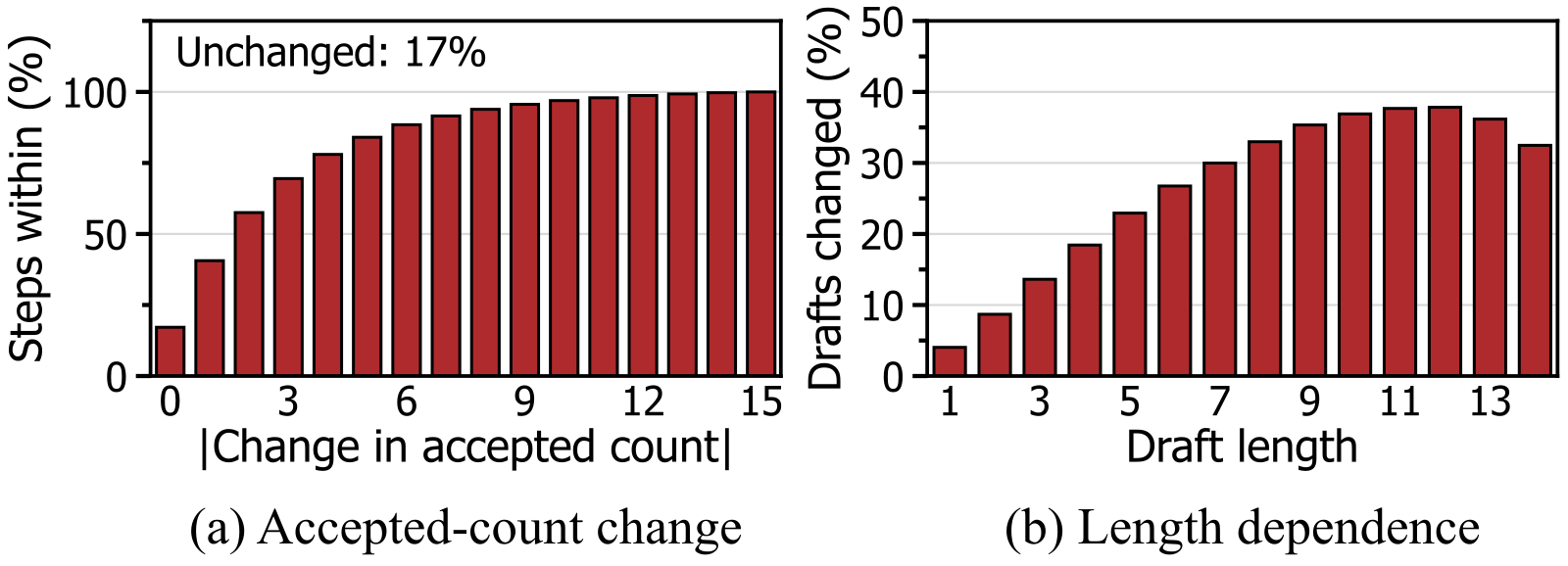
The right panel shows something else: a parallel drafter attends bidirectionally within its block, so the first 5 tokens of a 15-token draft differ from a 5-token draft about 23% of the time. ForeSpark therefore does not assume that a short draft is a prefix of a long one, and estimates each length separately; as shown later, on DFlash2 this step can actually be simplified.
Before drafting, estimate a triangle table from the target model's own state
ForeSpark splits each step into four stages, which the paper calls work-conserving speculation (WCS): drafting and verification compute is spent only where it pays off.
| Stage | Input | What it does | Output |
|---|---|---|---|
| Pre-draft estimate | From the verification pass that just finished: the context feature at the anchor (the last token confirmed in the previous step) and its embedding | A small low-rank network with one hidden layer | Acceptance probability for every position of every candidate length |
| Joint schedule | Estimates for the whole batch + latency tables profiled offline | Concave envelope, global sort, choose a plan by latency | Draft length D for each request, verification budget B for the batch |
| Variable-length draft | D | Pack all requests into one flat batch, each with only d_i empty slots | Draft tokens |
| Post-draft distribution | Hidden states of the drafts + path-selector features | Re-estimate survival probabilities, take the top B across the batch | Tokens actually sent to verification |
The pre-draft estimator ignores history and reads the target model's current context. Its output is a triangle: row d corresponds to "draft d tokens", and the j-th number in the row is the conditional acceptance probability of position j under that draft. With K=15 that is 120 numbers. Request B's table (illustrative) looks like this:
draft 1: 0.50                → expected accepted 0.5
draft 2: 0.40 0.50           → 0.4 + 0.2 = 0.6
draft 3: 0.70 0.71 0.60      → 0.7 + 0.5 + 0.3 ≈ 1.5
Multiplying each row's probabilities in order gives the survival probabilities, and summing those gives the expected number of accepted tokens. The paper's own example has survival probabilities 0.9, 0.7 and 0.3, which add up to 1.9. The estimator costs only a few matrix-vector products, so it can sit on the critical path between verification and drafting.
Look at B's third row: when drafting 3 tokens, the acceptance probability of position 1 rises from 0.5 to 0.7. The paper's Figure 6 draws exactly this case: a longer draft may lift the yield of earlier positions, so the reward curve need not be concave.
The reward curve is not concave, so cover it with a concave envelope first
Given each request's expected reward R(d) for drafting d tokens, the simplest approach is greedy: draft one more token while the next one's marginal gain is high enough. B's marginal gains are 0.5, 0.1 and 0.9 in turn. With a threshold of 0.3, greedy stops after 1 token because the second adds only 0.1, and so it misses the 1.5 that only a full 3-token draft brings.
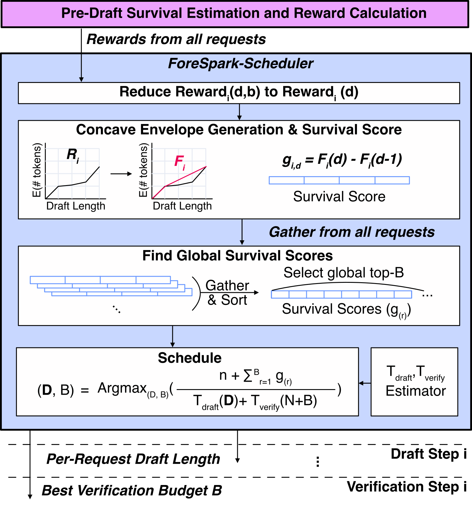
ForeSpark replaces each R with its concave envelope F: the smallest polyline above R whose marginal gains never increase. B's R is 0, 0.5, 0.6, 1.5; the straight line from the origin to (3, 1.5) already lies above the two middle points, so F is 0, 0.5, 1.0, 1.5, and each token's marginal gain (the paper calls it the survival score g) is 0.5. The large gain that only the third token brings is spread evenly over the tokens in between, so the selection does not stop early. A is already concave, so its envelope is unchanged and its g is 0.9, 0.7, 0.5; C's g is 0.3, 0.1, 0.05.
Next, sort the g values of the whole batch together:
0.9(A1) 0.7(A2) 0.5(A3) 0.5(B1) 0.5(B2) 0.5(B3) | 0.3(C1) 0.1(C2) 0.05(C3)Because each request's g never increases, the top entries are always a prefix of each request, and taking the top 6 directly gives D=(3, 3, 0). There is no search over 3³ combinations; with K=15 and hundreds of requests it is still a single sort. This is an approximation, and on real batches the paper measures it within 0.01% of the exhaustive optimum on average.
After sorting, put a price on drafting time
Sorting does not yet decide where to cut. DSpark treats drafting time as a constant when it picks the verification budget; ForeSpark makes it a variable and picks the D and B that maximize this ratio:
D decides which scores take part in the sort: each request has scores only for the first d_i positions it is scheduled to draft, and these scores are estimated by the predictor before drafting. B takes the top B of these positions by score for verification, so B cannot exceed ΣD. The numerator is one guaranteed token per request plus these top B scores; the denominator is the offline-profiled drafting latency plus verification latency, and N is the number of non-speculative tokens. At high load every extra drafted token slows the whole batch, so the cut moves forward and drafting is tight; at low load extra drafting costs almost nothing, so the cut moves back and drafting is generous. Full-block drafting with adaptive verification is one plan in this space, so at low load ForeSpark should not fall far behind DSpark. Hoot says

Illustrative: reusing the article's g ranking for A, B and C, n=3, drafting and verifying the top x scores (no over-drafting), with step latency 1 + c·x. At high load (c=0.2) the ratio peaks at the top 2 (about 3.29), so only A drafts 2 tokens; at low load (c=0.1) it peaks at the top 6 (about 4.1), which is exactly D=(3, 3, 0). Note that g is not the true per-position survival: B's first 2 g values sum to 1.0, while drafting 3 and verifying the first 2 is expected to yield about 1.2, and R(2) for a 2-token draft is 0.6. g is a planning score spread out by the concave envelope. So in the article's over-drafting illustration (A and B both draft 3, B=4), which 4 positions get verified is re-picked by the post-draft estimate: by g, A's third token (0.5) ties with B's positions and cannot be told apart; by the post-draft estimate, A's third is only 0.4 and B's second is 0.5, so the first 2 of both A and B are verified.
Source
paper §4.3 joint schedule (Eq. 4: sum of the top-B g over drafting plus verification latency, B no more than ΣD, over-drafting allowed); §4.4 post-draft estimator and budget distribution (verify the B positions with the highest post-draft survival across the batch); Figure 6B may be smaller than ΣD, meaning the scheduler deliberately over-drafts and leaves the extra candidates for the post-draft estimator to re-pick based on the tokens actually written. Illustration: when drafting is cheap, the scheduler lets A and B both draft 3 tokens but sets B=4. After drafting, the post-draft estimator re-estimates survival from each position's hidden state and DFlash2's path-selector feature, say 0.95, 0.8, 0.4 for A and 0.7, 0.5, 0.45 for B; the top 4 across the batch means A and B each verify their first 2. The pre-draft estimator can only guess from context, while the post-draft estimator sees the real drafts, which is why over-drafting a little helps. Verification is still standard speculative sampling, so the output distribution is unchanged.
The search is cheap because the drafter and the target replay CUDA graphs in a few token-count buckets; latency is constant within a bucket, so each pair of buckets needs only one candidate.
Same checkpoint, over 60% less drafting time
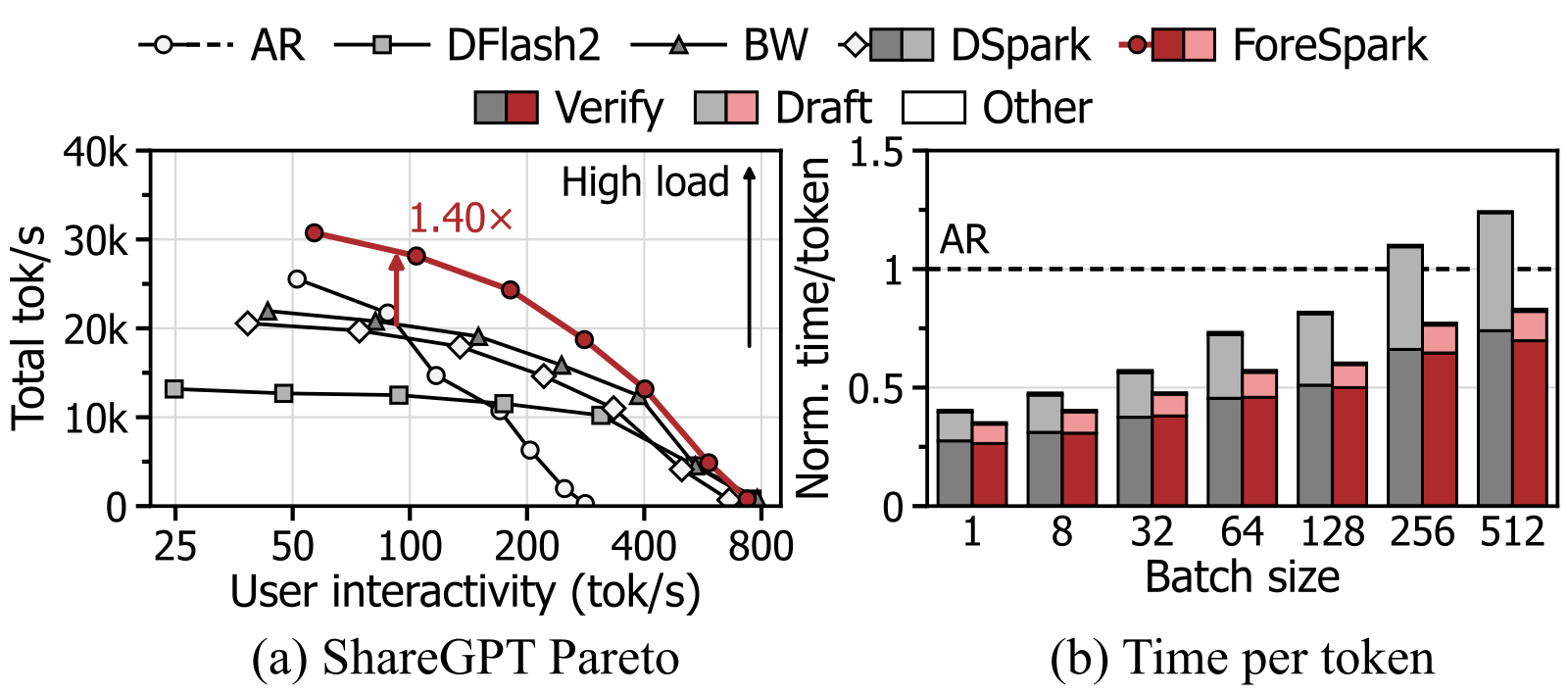
The experiments run on vLLM with the dense Qwen3-14B plus the MoE models GLM5.3-Flash (320B, 18B active) and GLM5.3 (744B, 40B active), comparing total throughput at the same per-user speed. The baselines are AR (no speculation); DFlash2 (draft everything, verify everything); BW; DSpark; and ForeSpark w/o JS (JS stands for joint scheduling), which uses ForeSpark's own checkpoint but removes the pre-draft estimator and joint scheduler, falling back to full drafting plus adaptive verification. This last baseline matters most, because ForeSpark's drafter is built on DFlash2 and does not share DSpark's backbone.
On ShareGPT-Decode, which measures only the decode phase, ForeSpark reaches up to 1.77/1.40/1.34x the throughput of DSpark (for the three models in order) and 1.37/1.46/1.46x that of w/o JS. This shows the gain is mainly not from a different backbone: with the same checkpoint, adding joint scheduling alone gives roughly 1.4x.
The time breakdown makes the accounting more direct. At the largest batch, ForeSpark spends 62/70/76% less time drafting than w/o JS and 76/68/67% less than DSpark. On Qwen3-14B, DSpark and w/o JS take 1.41x and 1.14x the time per token of AR, while ForeSpark takes 0.89x. This shows the saving is mainly drafting time: with the same checkpoint, joint scheduling turns time per token from slower than AR into faster than AR.
The scheduler itself also has to be fast. On GLM5.3-Flash with 192 requests, ForeSpark makes a decision in 88 μs, while an exhaustive scheduler with the same inputs needs 8.2 ms; at batch sizes 64 and 192 the exhaustive scheduler's throughput even falls below the version with adaptive verification only (that is, w/o JS). This shows the benefit of joint scheduling rests on being cheap: the most exact but slow scheduler gives the gain back.
The estimator is indeed more accurate than history. Over 1.48M full-block drafts, ForeSpark predicts the acceptance length within 1 token for 60% of drafts, against 41% for the previous step's acceptance count. Under latency SLOs, ForeSpark sustains up to 1.51x the request rate of DSpark.
Gains concentrate at high load, and there are costs
The gains come mostly from high load. At a batch size of 1, ForeSpark's per-user speed is 0.96 to 1.15x that of DSpark, essentially on par. On the end-to-end workload (ShareGPT-E2E) the gain is smaller, because prefill tokens share each step with decoding, and scheduling cannot remove these non-speculative tokens. In the heaviest load setting of Qwen3-14B Decode, AR still has the highest throughput, and ForeSpark is only the speculative method that comes closest to it.
Nor do the gains come from a stronger drafter: without adaptive verification, mean acceptance length on the three models is within 3.2% of DSpark and equal to DFlash2, and the two estimators add only 0.1% to 0.2% parameters. Another counterintuitive result: on DFlash2, replacing the per-length estimates with a single length-15 curve (ForeSpark-SC in the paper) predicts acceptance just as accurately and matches throughput. So per-length estimation is not necessary on this drafter; the authors keep it so the method also works on drafters where "a short draft is a prefix of a long one" does not hold.
Back to request C in the illustration: the global sort may leave it with no draft at all in a step. Outputs are unaffected, but speedups become uneven across requests, and the authors suggest a per-request minimum budget to fix this. In addition, both estimators are conservative relative to an oracle that knows the true acceptance, partly because they are calibrated only on Alpaca.
Back to the accounting from the start: a parallel drafter cannot change its length while drafting, so ForeSpark moves the decision before drafting. It estimates each length's yield from the target model's current state, and sets the whole batch's draft lengths and verification budget together in one sort. The 1.77x is relative to DSpark and includes the backbone difference; with the same checkpoint, joint scheduling alone brings 1.37/1.46/1.46x.
How did this read for you?
Hoot made a note. Thanks for the feedback.

One tap, no sign-in; tap again to undo. Only anonymous counts are kept, never who you are.
Related papersMore from Paper Daily
 Infra · 2026-11-02TableTune: Measured, Self-Correcting Draft-Length Tables for Dynamic Speculative DecodingThe table in vLLM's documentation that sets how many tokens speculative decoding guesses per step at each batch size can visibly cut throughput on a different GPU or model. This paper gives a tool that measures the best table in minutes and keeps correcting it as traffic changes. Speculation only pays while the GPU has spare compute, so the more requests share a batch, the fewer tokens each step…
 Infra · 2026-11-13Multi-Future Drafting: Mixture Block Drafters for Tree-Verified Speculative DecodingIn speculative decoding, a drafter that drafts a whole block of tokens in one forward pass is fast, but it gives each position its own separate distribution. When the continuation has two equally plausible phrasings, a draft tree ranked by multiplying per-position probabilities splices them into sentences the target model would never say. The authors prove that such a tree can hold both phrasings…
 Infra · 2026-11-05HybridSpec: Throughput-Aware Speculative Decoding for Hybrid GDN-MoE ModelsWhen doing speculative decoding on models that mix Gated DeltaNet (GDN, a linear-attention layer with a recurrent state) and MoE layers, how many draft tokens to verify per round cannot be copied from dense-model settings. On one hybrid Qwen model, raising the tokens verified per round from 4 to 16 makes verification 71% slower. Each round, HybridSpec scores every candidate length: the tokens it…
 Infra · 2026-10-27NgramRL: Accelerating RL Post-Training for Structured Generation via Rollout-Aware N-gram Speculative DecodingIn LLM reinforcement learning post-training, generating answers often takes over 70% of training time. This paper notices that the answers a prompt received in recent training rounds closely resemble what it will produce now, so they make good drafts. NgramRL builds an n-gram draft table for each prompt from only its own recent answers. During generation, the last few tokens of the current answer…
 Infra · 2026-10-23RCSD: Reinforcement and Continual Learning for Domain-Specific Speculative DecodingHisense's RCSD continues training a speculative-decoding draft model that was distilled with HASS, using DPO or GRPO: sequences from the target alone are "good," sequences alternating target and draft are "bad," and the GRPO variant scores by acceptance rate. On Qwen3-1.7B and Llama-3.1-8B, acceptance length exceeds HASS on four datasets and draft steps 3–6—for example Qwen3-1.7B on GSM8K at step…
 Infra · 2026-11-04Fairway: Load-Aware KV Cache Reuse for LLM Prefill SchedulingPrefill queueing under a prefix cache can keep both the median latency low and the tail short. While the queue is short, serve cheap requests with long cache hits first; move a request forward the longer it has waited relative to its own prefill time; and cap how much work cheap requests may place ahead of the oldest request. This is what Fairway does. Agent and RAG requests often share a prefix,…
 Infra · 2026-11-03LEAP: Efficient LLM Inference Scheduling with Generalizable Length PredictionRunning short requests first clearly lowers average latency, but only if you know roughly how long each request will generate, and existing length predictors rank worse when the domain changes while costing GPU time of their own. LEAP finds that the hidden states the serving model computes during prefill already carry an output-length signal, and a single linear layer on one layer's hidden state…
Discussion
Add experiment details, reproduction notes or a different take. Requires a GitHub sign-in.
Loading the discussion…