Contents · 9 sections
1What problem is it actually solving?2The big picture: pick a length first, revise it once after the first router3How the length is picked: extra tokens weighed against extra time4Routing correction: decide on the extra token after seeing the real expert assignment5The GDN state: compute in one go, rebuild at the kept length afterwards6How well does it work?7Limitations as I see them8How an inference team could try it9VerdictSHARE

When doing speculative decoding on models that mix Gated DeltaNet (GDN, a linear-attention layer with a recurrent state) and MoE layers, how many draft tokens to verify per round cannot be copied from dense-model settings. On one hybrid Qwen model, raising the tokens verified per round from 4 to 16 makes verification 71% slower. Each round, HybridSpec scores every candidate length: the tokens it expects to produce, estimated from drafter confidence, minus the tokens that the verification time would yield at the average speed. At the target model's first MoE router, it checks how many new experts one extra token would activate, adds that cost to the score, and verifies the extra token only if it pays off. On three such models, with the same DFlash drafter, it runs about 1.3 times as fast as vanilla DFlash, which verifies every draft. Teams doing speculative decoding on hybrid models should read it, because a verification length tuned on dense models wastes a lot of time there.
What problem is it actually solving?
DFlash drafts in parallel: one forward pass gives 15 draft tokens. Drafting takes about 1.8 ms, only a fraction of the target's verification time. The bulk of each round becomes the target's verification. The paper calls the number of tokens the target processes in a round the verification length: the newest confirmed token plus the drafts being checked. Vanilla DFlash verifies all 15 drafts every round, a verification length of 16.
A small example (illustrative) shows where the waste is:
| This round (illustrative) | Verification length | Drafts kept | Drafts still checked after the wrong one |
|---|---|---|---|
| The 4th draft is wrong, verify all | 16 | 3 | Drafts 5 to 15, 11 in total |
| Same drafts, verify only the first 5 | 6 | 3 | Only draft 5 |
The system does not know in advance that the 4th draft is wrong. The second row only shows that a shorter length wastes less.
On dense models this waste hardly matters. At batch size one, a dense model spends most of its time reading weights from memory, so a few extra tokens add almost no time. The authors measured Qwen3-4B: going from length 4 to 16 makes verification only 4% to 6% slower.
Hybrid models are different. Models such as Qwen3.5 and Qwen3.6 are mostly GDN layers (30 of the 40 layers of Qwen3.6-35B-A3B) with a few ordinary attention layers mixed in, and every layer ends with an MoE block. On Qwen3.6-35B-A3B, the same step from 4 to 16 makes verification 71% slower, almost all of it in the GDN and MoE layers. There are two reasons:
- The GDN state must be able to roll back. GDN keeps no growing KV cache. It keeps a fixed-size state matrix and updates it with every token it reads. During verification it is not known how many drafts will be kept, so SGLang by default stores a full copy of the state after every update, to roll back to the accepted position. The longer the verification, the more copies.
- MoE cost depends on how many experts are used. These models send each token to only 8 of 256 experts. One more verified token adds almost no time if its experts were already used by earlier tokens. If it activates new experts, another set of expert weights must be read. Which token uses which experts is known only once the target actually runs.
So on hybrid models the verification length can no longer be fixed at 16. One pre-measured average latency curve is not enough either, because how many new experts the extra token activates is known only once the target runs.
The big picture: pick a length first, revise it once after the first router
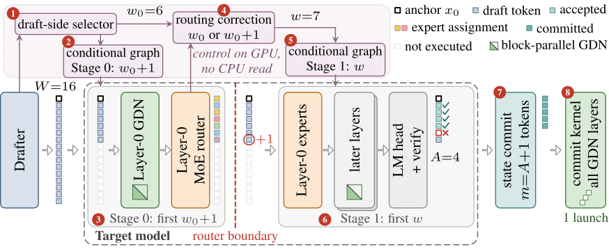
One round of HybridSpec splits into four steps:
- The draft side picks a length first. After the draft model outputs 15 drafts, the confidence of each draft is used to estimate the probability that the first 1, the first 2, ..., the first 15 drafts are all kept. Combined with a pre-measured relation between verification length and target latency, it picks the most worthwhile length, written . These probabilities are only predictions; whether a draft is kept is known only after the target has run.
- The target runs a short piece first. The target takes the first tokens plus one extra, runs them through the Layer-0 GDN layer and MoE router, then pauses. If all 16 are already selected, or the remaining output budget is too small, no extra token is carried and no correction is made. At this point the expert assignment of every token is known, but no expert has run yet. The paper calls this pause the router boundary.
- Routing correction. It counts how many new experts the extra token uses in Layer 0, re-estimates its latency from that count, and then keeps or drops it. The final verification length is or .
- Finish on the selected tokens only. Starting from the Layer-0 experts, it runs to the last layer, checks the drafts, and writes the kept tokens into each cache. Nothing already computed in Layer 0 is recomputed.
The key division of labour is: the draft side makes the main decision from the drafts' confidence, and the router boundary makes one small correction from the real expert assignment. The length stays on the GPU throughout; neither choosing it nor launching computation by it needs a CPU read. The authors record one CUDA Graph in advance for every possible length of the first stage and of the second stage, and at run time a conditional node launches the right one directly from the length on the GPU. Now the pieces one by one.
How the length is picked: extra tokens weighed against extra time
Why not cut at "acceptance probability above some threshold"? Because the goal is total throughput over a whole generation: all tokens produced across rounds divided by total time. This overall ratio is not the average of per-round ratios, so the best choice in one round depends on how fast the whole run can go. The authors use Dinkelbach's theorem to turn it into a score for each round:
is the estimated probability that the first drafts are all kept, so the sum is how many tokens this round is expected to produce. is the target's latency curve: per-round time measured at several fixed lengths, then fitted into one curve over length. is the throughput the whole generation is expected to reach, that is, tokens produced per millisecond on average, estimated beforehand on calibration data. The score means: in the same time, the average rate would have produced times that time in tokens, so the extra verified tokens must be expected to beat that to pay off. The selector scores every length from 2 to 16 and takes the highest. The measured latency curve is not always smooth, so it cannot stop at the first unfavourable comparison. Hoot says

The score is the expected tokens produced minus the tokens the same time would yield at the average speed. Illustrative: each extra draft is kept with probability 0.8 times the previous one. When cost grows slowly (dashed), verifying all 16 scores best. When cost grows fast (solid), 6 scores best and verifying all 16 is nearly wasted. Drag the slider to see each length's score.
Source
illustrative example of the paper's §3 length score (Eq. 5)A mental-math example (illustrative): suppose that, through , the time of each extra verified position is worth 0.3 tokens. The cumulative acceptance probabilities of the first 4 drafts are 0.9, 0.7, 0.5 and 0.25. Verifying the 3rd draft still pays, since 0.5 is above 0.3; the 4th is worth only 0.25 and does not. In this simple case where every position costs the same, the highest score is to verify 3 drafts; adding the confirmed token at the start, the verification length is 4.
Where do the acceptance probabilities come from? The draft model gives each draft token a top-1 confidence and an entropy. In the calibration phase, the authors learn two things on 280 calibration prompts: a map from confidence to acceptance probability, and a small logistic model. The logistic model's inputs are the mapped confidence, the position, the entropy, and whether the entropy at this position rose or fell relative to the earlier positions. At inference, each round, this round's 15 confidences and entropies are plugged in to get a conditional probability for each position: the probability that this draft is kept, given that all earlier drafts were kept. Multiplying the conditional probabilities of positions 1 to gives , the probability that the first drafts are all kept. This step uses only the draft model's own outputs and finishes before the target starts.
Routing correction: decide on the extra token after seeing the real expert assignment
When the draft side picks a length, the target has not run yet, so it can only charge the average expert cost from calibration. Whether the extra token will actually activate new experts is not known in advance.
HybridSpec's answer is to let the target carry one extra token and run it up to the Layer-0 router. The router has already assigned this token's experts, so it can count how many new experts the token uses in Layer 0. The authors measured in the appendix that expert assignments in later layers are moderately correlated with Layer 0 (a correlation of about 0.5), so the Layer-0 count of new experts helps estimate the later layers. Concretely, calibration first builds a table: at this position, for tokens that used 0, 1, 2, ... new Layer-0 experts, how many new experts they used on average in the later layers. At inference the Layer-0 count of new experts is looked up in this table, giving how many new experts the token is expected to use across all MoE layers.
At batch size one, each expert handles only a few tokens, and MoE time depends mainly on how many distinct experts are used. The authors measured that on the two 35B models each extra distinct expert adds about 4.18 microseconds. The re-estimated time is computed like this: start from the curve's time for verifying one more token, and deduct the Layer-0 part already computed for it; then, for each new expert the table gives above this position's average, add 4.18 microseconds, and for each one below, subtract it.
The correction reuses the same score. Adding this token raises expected output by , the estimated probability that the earlier drafts and this one are all kept. If that number is higher than its re-estimated extra time (converted into tokens with the same ), it is kept; otherwise it is dropped.
An example (illustrative): the draft side picked 6, and the extra 7th token uses Layer-0 experts all already used by the first 6. It adds almost no expert cost, and Layer 0 has already been computed for it. As long as this probability is high enough (assume it is here), the re-estimate says it pays off and 7 are verified. If it uses several new experts, the re-estimated time goes up, it is dropped and only 6 are verified. The correction adds at most one token, because Layer 0 must compute every token that might be added in every round, and each extra one is a fixed cost.
The GDN state: compute in one go, rebuild at the kept length afterwards
The GDN problem is rolling the state back. The default updates the state token by token and stores a full state matrix after every update. HybridSpec uses one fact: during verification all tokens of the round are already known.
Each time GDN reads a token, it first multiplies the old state by a decay factor, then writes a change : it reads the old value stored under this token's key and moves it toward this token's value by a fraction (the delta rule). The change of token depends on the state before it, and so on the earlier tokens' changes and the round's starting state . Stacking all changes into a matrix turns these dependencies into one lower-triangular linear system. The right-hand side is each token's value minus what its key reads from the decayed , times . The coefficient matrix has ones on the diagonal, and entry for is times the decay between the two tokens times the inner product of their keys. One solve gives every token's change, and token 's output reads state with its own query. is assembled from and the changes of tokens 1 to by the same formula used below to rebuild the state, so it uses only its own and earlier changes. This is the standard chunkwise-parallel algorithm used in training.
After the solve, the kernel stores no per-step state. It keeps three small things per token: its key, its change, and the cumulative decay up to it. Once checking is done and tokens are known to be kept, the state at the kept position is rebuilt as:
is the state at the start of the round, and are token 's change and key, and is the log of the cumulative decay. The intuition: the starting state is multiplied by the decay of the whole stretch, and each kept token's change is multiplied by the decay that the tokens after it bring, then added in.
Keeping only these three things and rebuilding afterwards was already used by earlier work such as SpecLA and TreeWY. What is new in HybridSpec is fused kernels optimised for single-request verification, and one launch that rebuilds the state of every GDN layer.
Measured alone on the 30 GDN layers of Qwen3.6-35B-A3B with every draft kept, these kernels run at 1.54 to 4.04 times the speed of the SGLang default kernels at lengths 4 to 16. The longer the length, the larger the saving, because the default stores one more state per token. They also save memory: at batch size one the default reserves 1.88 GB to store every step's state, 40% of the size of the attention-cache pool; HybridSpec needs none of it.
How well does it work?
The authors tested three GDN plus MoE models in SGLang on A100s, each with its official DFlash draft model, one request at a time, greedy decoding. Prompts come from 7 categories of SPEED-Bench, 280 for calibration and another 280 for testing. The table gives the average over the 7 categories; speedup is relative to the target generating token by token on its own:
| Target model | Vanilla DFlash | EVICT (strongest baseline) | HybridSpec |
|---|---|---|---|
| Qwen3.5-35B-A3B | 1.45× | 1.59× | 1.88× |
| Qwen3.6-35B-A3B | 1.37× | 1.51× | 1.83× |
| Qwen3.5-122B-A10B | 1.32× | 1.65× | 1.75× |
All methods use the same DFlash drafter; vanilla DFlash means verifying all 15 drafts every round. HybridSpec is fastest on every category of every model, at 1.30 to 1.33 times the speed of vanilla DFlash.
Interestingly, it produces fewer tokens per round than vanilla DFlash. On the two 35B models it verifies only 6.4 and 6.2 tokens per round on average, versus a fixed 16. Tokens produced per round therefore drop by about 5%, but time per round falls from about 23 ms to 16.3 to 16.5 ms, so overall it is still faster.
Most of the drafts it skips would have been rejected anyway. This comes from comparing afterwards: of the 9.6 to 9.8 drafts per round left unverified, fewer than 3% would have been kept. So the skipped part costs almost nothing.
Which part contributes most? On Qwen3.6-35B-A3B the authors remove one component at a time:
| Component removed | Replaced by | Mean verification length | Speedup | HybridSpec faster by |
|---|---|---|---|---|
| Length selection | Calibrated fixed length 7 | 7 | 1.54× | 1.19× |
| Length selection | Fixed length 16 | 16 | 1.46× | 1.25× |
| Routing correction | Draft-side choice only | 6.1 | 1.73× | 1.06× |
| GDN kernels | SGLang default kernels | 6.2 | 1.74× | 1.05× |
So per-round length selection is the big one. Note that removing length selection also removes two-stage verification and the routing correction, and both fixed-length variants use the new GDN kernels. Compared with fixed length 7, it verifies fewer on average (6.2 vs 7) yet produces more per round (4.57 vs 3.99), because rounds that deserve long verification get it and others stay short. The routing correction adds about 6% more, and the new kernels about 5% more.
On generalization: without recalibration, on 4 other SPEED-Bench categories not used for calibration, the mean speedup is 1.69×, versus 1.31× for vanilla DFlash. This shows the calibrated selector is not just fitted to those few categories.
With temperature-one sampling on the two 35B models, HybridSpec reaches 1.57× and 1.60×, versus 1.20× and 1.21× for vanilla DFlash. So the advantage does not depend on greedy decoding.
Limitations as I see them
First, the main results are all single-request. The appendix version with 4 concurrent requests has only 10% more throughput than vanilla DFlash (497 vs 451 tokens per second). The reason is that one batch must share one verification length picked from 5 candidates, which cannot fit each request. The paper only tests up to 4 concurrent requests; my guess is that the gain shrinks further at larger batches. On the other hand, the new kernels store no per-step state, so with 4 concurrent requests the cache holds 9.8 times as many tokens as vanilla, a real benefit for serving.
Second, hardware and models are narrow. Only A100s were tested, all three models are Qwen GDN plus MoE models, and the draft model is always DFlash. The latency curve and the conversion rate must be measured and calibrated on the specific runtime, so a new GPU or inference engine means redoing them.
Third, the code is not out yet. The authors say they will release it upon acceptance; the new kernels and conditional CUDA Graphs are substantial engineering, so reproducing it yourself takes real effort.
How an inference team could try it
- Measure a latency curve first. On your own hybrid model, fix the verification length at several values between 2 and 16 and measure verification time per round. If the curve is flat, the bottleneck is still weight reading and there is no hurry to change anything.
- Start with the cheapest version: find one best fixed verification length on calibration data. In the paper fixed length 7 is faster than fixed 16 (1.54× vs 1.46×), but both numbers already use the new GDN kernels; the effect of tuning the length alone without the new kernels was not measured.
- Then add per-round length selection. Estimate acceptance from the draft model's confidence and entropy, pick the length with the score above, and see whether throughput improves further.
- If the target has GDN layers, consider replacing the verification kernels last; they also free the memory used to store states.
Verdict
On hybrid models, the verification length is a choice to be costed round by round, counting both the chance that drafts are kept and the real cost of the target verifying one more token.
| Dimension | Assessment |
|---|---|
| Importance of the problem | Medium-high. More new open models use GDN plus MoE, and verification cost eats into single-request speculative decoding |
| Novelty of the method | Medium-high. Pausing after the first router to revise the length from the real expert assignment is a new angle |
| Strength of evidence | Medium. Three models, 7 categories and complete ablations, but only A100 and single-request; the batched gain is small |
| Engineering cost | Medium-high. Needs conditional CUDA Graphs, two-stage verification and new GDN kernels; code not yet released |
| Worth trying? | Yes for fixed-length calibration and per-round selection; wait for the code before the kernel part |
How did this read for you?
Hoot made a note. Thanks for the feedback.

One tap, no sign-in; tap again to undo. Only anonymous counts are kept, never who you are.
Related papersMore from Paper Daily
 Infra · 2026-10-27NgramRL: Accelerating RL Post-Training for Structured Generation via Rollout-Aware N-gram Speculative DecodingIn LLM reinforcement learning post-training, generating answers often takes over 70% of training time. This paper notices that the answers a prompt received in recent training rounds closely resemble what it will produce now, so they make good drafts. NgramRL builds an n-gram draft table for each prompt from only its own recent answers. During generation, the last few tokens of the current answer…
 Infra · 2026-11-13Multi-Future Drafting: Mixture Block Drafters for Tree-Verified Speculative DecodingIn speculative decoding, a drafter that drafts a whole block of tokens in one forward pass is fast, but it gives each position its own separate distribution. When the continuation has two equally plausible phrasings, a draft tree ranked by multiplying per-position probabilities splices them into sentences the target model would never say. The authors prove that such a tree can hold both phrasings…
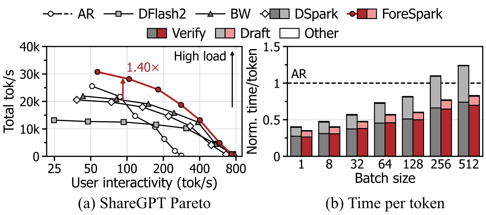 Infra · 2026-11-12ForeSpark: Joint Draft and Verification Budget Scheduling for Parallel Speculative DecodingA parallel draft model writes a whole block of draft tokens in one forward pass. Current systems write the full block first, then pick the most promising few for the target model to verify. The authors find this wasteful under high load: drafting takes up to 40% of each step, and most of what is drafted is thrown away without ever being verified. The difficulty is that a parallel draft model must…
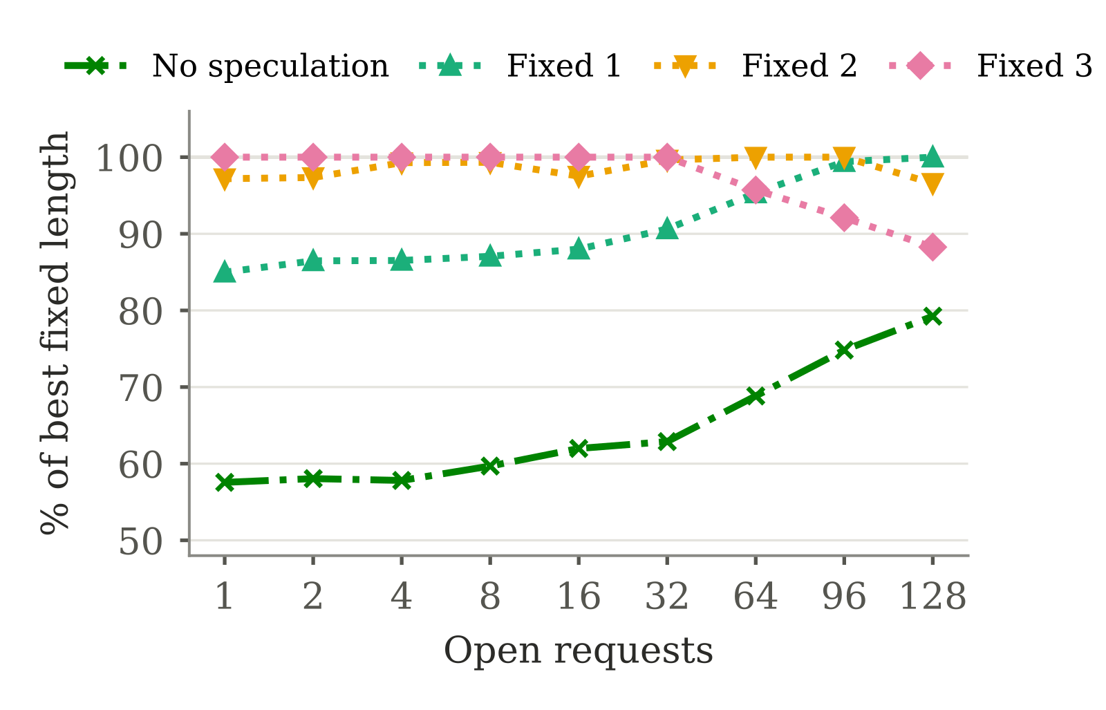 Infra · 2026-11-02TableTune: Measured, Self-Correcting Draft-Length Tables for Dynamic Speculative DecodingThe table in vLLM's documentation that sets how many tokens speculative decoding guesses per step at each batch size can visibly cut throughput on a different GPU or model. This paper gives a tool that measures the best table in minutes and keeps correcting it as traffic changes. Speculation only pays while the GPU has spare compute, so the more requests share a batch, the fewer tokens each step…
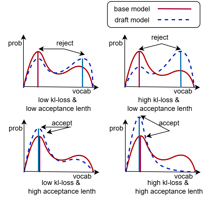 Infra · 2026-10-23RCSD: Reinforcement and Continual Learning for Domain-Specific Speculative DecodingHisense's RCSD continues training a speculative-decoding draft model that was distilled with HASS, using DPO or GRPO: sequences from the target alone are "good," sequences alternating target and draft are "bad," and the GRPO variant scores by acceptance rate. On Qwen3-1.7B and Llama-3.1-8B, acceptance length exceeds HASS on four datasets and draft steps 3–6—for example Qwen3-1.7B on GSM8K at step…
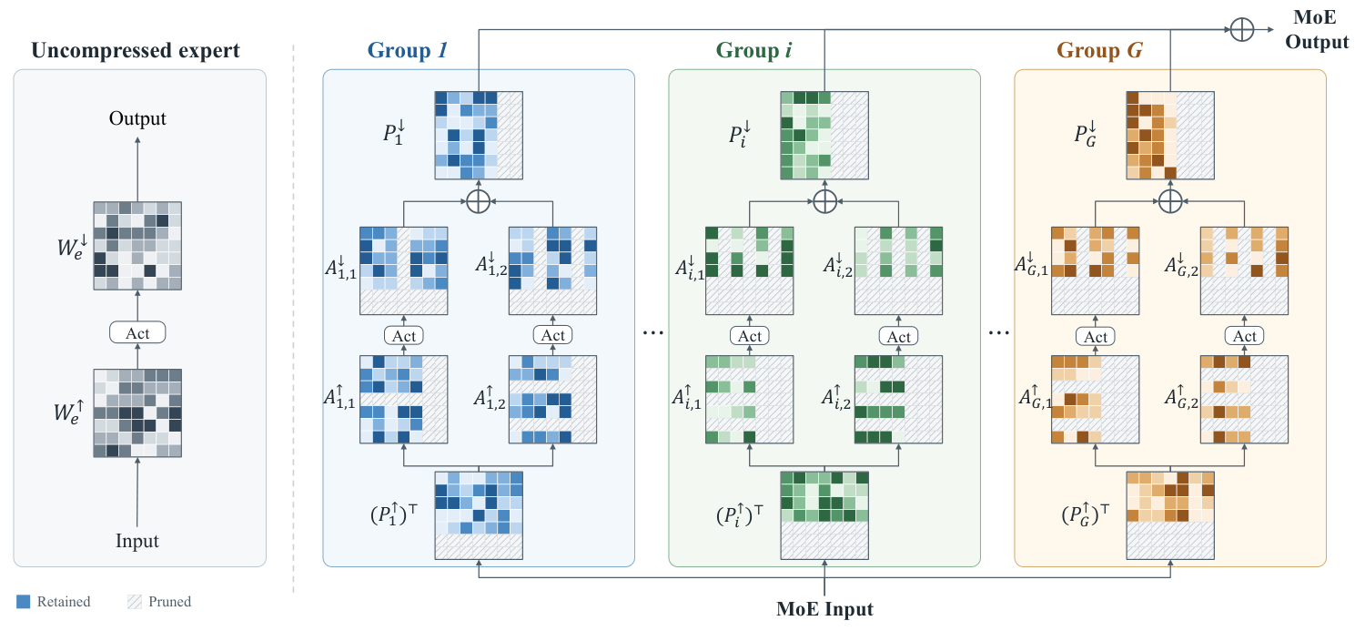 Infra · 2026-10-26GS-MoE: Training-Free MoE Compression via Groupwise Subspace Sharing and PruningMixture-of-experts (MoE) models activate only a few experts per token, so compute is cheap, but every expert's parameters must stay in GPU memory, and memory is usually the first thing that blocks deployment. This paper proposes GS-MoE, which needs no retraining and compresses experts along two axes at once. First, similar experts are grouped, and each group shares one input and one output projec…
 Infra · 2026-11-05Look Before You Launch: Learned Throughput Prediction for Hardware Selection in a Production Training FleetThe same training job can often run on several accelerator types, and which one is cheapest depends on its throughput on each. A job placed on the wrong type still finishes without any error, so the extra cost goes unnoticed. LEAP, a hardware-selection service the authors run in a production fleet, predicts a job's throughput on every candidate type at submission time, then ranks the types by pre…
 Infra · 2026-10-25ATTUNE: Agentic Throughput Tuning for LLM TrainingMove a large model to a different GPU or framework version, and the training recipe that used to be fastest often no longer is. The recipe settles how the model is split across GPUs, which low-level routines to use, and how GPU data transfers overlap with computation. ATTUNE lets an AI agent able to write code and run commands tune recipes, given a recipe that runs and a budget of GPU-hours; it t…
Discussion
Add experiment details, reproduction notes or a different take. Requires a GitHub sign-in.
Loading the discussion…