Contents · 8 sections
1Are two items whose last three SID tokens match actually similar?2What steps does an item go through, from title and description to being recommended?3How many branches should each group get?4If a group that looks good in embedding space gets no purchases, how does the model learn it?5With the same model and the same embeddings, how much difference does the code alone make?6Does the gain come at the expense of unpopular items?7How much do adaptive branching and the interaction requirement each contribute?8What needs tuning for a different catalog?SHARE

When you build the codes a recommender generates for its items, the later digits only mean something after the earlier ones, so this paper groups items layer by layer into a tree and uses the tree path as the code; with the recommender unchanged, Recall and NDCG average about 13% above the strongest baseline.
Generative recommendation does not score each item separately. The recommender reads a user's history and writes the code of the next item one token at a time, and that code is called a Semantic ID (SID). This article uses one illustrative beauty store throughout: it has 36 items in three categories, lip makeup, skincare, and perfume. A user has just bought a matte lipstick, and the model must write the SID of the next item, for example <c0_0><c1_1><c2_0>. The system then looks up the SID-to-item table to turn that token string back into an item.
Items do not come with SIDs. A separate step has to build one for every item before the recommender is trained, and the recommender can only learn from those SIDs afterward. If the first token of an SID corresponds to a broad category, writing it amounts to computing one probability each for lip makeup, skincare, and perfume, and the second token then subdivides the chosen category. The difficulty is this: suppose two very similar lipsticks get SIDs that start differently. After a user buys a matte lipstick, either one could be next, so the model has to spread probability across two different first-token values and cannot concentrate it on one.
The most common construction today is residual quantization, represented by the RQ-VAE used in TIGER. Given an item's embedding, RQ-VAE first finds the nearest center in the first codebook (a table holding a number of center vectors) and records that center's index as the first token. RQ-VAE then subtracts this center from the item embedding and takes the remaining difference (the residual) to the second codebook to find its nearest center again. The whole store shares the second codebook, so every item looks up the same one no matter what its first token is.
Illustration: a matte lipstick has embedding (1.0, 0.2), and subtracting the center (1.0, 0) leaves the residual (0, 0.2). A woody perfume has embedding (0, 1.2), and subtracting the center (0, 1.0) also leaves the residual (0, 0.2). The two residuals are identical, so they find the same nearest center in the second codebook and get the same second token, even though the lipstick and the perfume are far apart in the original embedding space.
Some methods do assign codes along a tree, such as SEATER (a tree method that builds SIDs hierarchically and then refines them with contrastive learning), but in tree-based methods of this kind the number of parts each group splits into (the branching factor) is usually fixed in advance. In this store (illustrative), there are only 8 perfumes, with just two scent families, floral and woody, so 2 branches are enough. If every group must split into 4 branches, the perfumes must also be cut into 4, and floral perfumes end up in different branches. This paper targets exactly these two gaps. For items whose second tokens match while the items themselves are not close, it makes every SID token represent one grouping choice on a tree. For the fixed number of branches, it lets each group's branch count depend on how many clusters that group forms in embedding space.
Are two items whose last three SID tokens match actually similar?
The authors first test a hypothesis: if each position of an SID has its own independent meaning (for example, if the second token denotes the same attribute no matter what precedes it), two items with the same last three tokens should be very similar. The authors use TIGER's RQ-VAE to generate 4-token SIDs for the items in the Beauty dataset, select item pairs by the matching patterns in the table below, and compute the mean cosine similarity of the pairs under each pattern. A pattern is written in 0s and 1s, so 1100 means the two items share the first two tokens and differ in the last two.
| Position-by-position matching pattern of the two SIDs | Mean cosine similarity | Mean cosine similarity of random item pairs in the same analysis |
|---|---|---|
| 1000: only the first token matches | 0.758 | 0.554 |
| 1100: the first two tokens match | 0.874 | 0.554 |
| 1110: the first three tokens match | 0.920 | 0.554 |
| 1000: only the first token matches | 0.740 | 0.570 |
| 0111: the first token differs, the last three match | 0.582 | 0.570 |
The first three rows and the last two rows come from two separate analyses, each estimating the means by sampling, and the estimates are not identical, so the 1000 pattern has two values, 0.758 and 0.740. When reading the table, compare each row only with the random pairs from the same analysis.
The first three rows show that the longer the run of matching tokens at the start of an SID (the prefix), the more similar the two items are, with similarity rising from 0.758 to 0.920. The last two rows show that pairs sharing only the first token reach 0.740, while pairs matching on the last three tokens but differing on the first reach only 0.582, nearly the same as the 0.570 of random pairs. The lipstick and perfume in our store, with different first tokens, the same second token, and items far apart, are the same kind of case as the 0111 row.
When the first tokens differ, matching later tokens says almost nothing about whether two items are alike; what a later token means depends on the tokens before it.
This measurement covers only the Beauty dataset and one construction, RQ-VAE. Longer prefixes meaning more similar items indicates that an SID subdivides items more finely token by token, like walking down a tree. The method the authors draw from this is direct: first group the items layer by layer into a tree, then read each item's path from the top of the tree to its own small group as its SID. They call this method AST (Adaptive Silhouette Tree, which groups items layer by layer starting from the whole store, with each group choosing its own number of branches).
What steps does an item go through, from title and description to being recommended?
| Step | Input | Operation | Output | When |
|---|---|---|---|---|
| 1 | An item's title, categories, and description | Concatenate into one text, encode with Qwen3-Embedding-0.6B, and normalize | One embedding per item | While building SIDs |
| 2 | The embeddings of one group of items | Try several branch counts, group with KMeans and score each (scoring is covered in the next section), and pick the highest-scoring split | The group split into branches | While building SIDs |
| 3 | Each resulting branch | Repeat step 2 until all tokens except the last are set, or until the group has no valid split | Every token except the last for each item | While building SIDs |
| 4 | The items in one small group at the bottom of the tree | Rank by item ID and write the rank as the last token | Each item's complete SID | While building SIDs |
| 5 | The SID sequence of a user's history and the SID of the next item | A T5 encoder–decoder learns to write the next SID from the history | A trained recommender | During training |
| 6 | The history of the user being served | The model writes SIDs token by token, and beam search keeps the few highest-scoring ones | Several SIDs, looked up to get items | During inference |
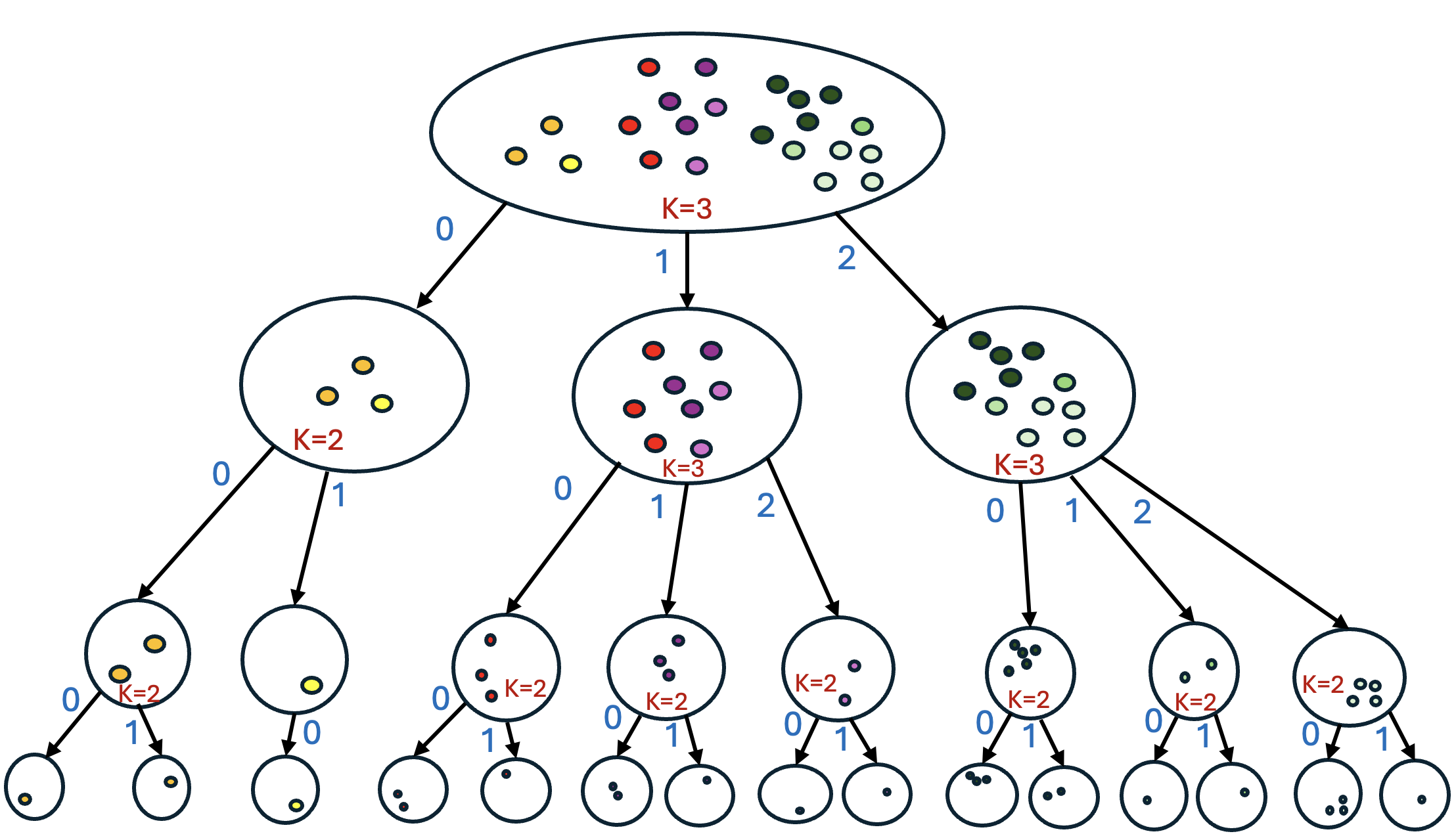
Back in the store, here is how a matte lipstick A gets its SID (illustrative). The whole store splits into three groups, A goes to group 0 (lip makeup), and the first token is <c0_0> (c0 marks the first position, and the 0 after it is the group number). The lip makeup group splits again, A goes to group 1 (matte), and the second token is <c1_1>. The matte group has 3 lipsticks, A ranks third by item ID, which is 2 when counting from 0, so the last token is <c2_2>.
So A's SID is <c0_0><c1_1><c2_2>, and a woody perfume's SID might be <c0_2><c1_1><c2_0> (group 2 is perfume, and group 1 under perfume is woody). The second token of both SIDs is <c1_1>, which means matte after lip makeup and woody after perfume. One training example takes a user's history of SIDs as input, for example just A, and its target is the SID of another lipstick in the same group, <c0_0><c1_1><c2_0>.
AST without the interaction requirement writes closeness directly into the structure of the SID. The items under one prefix are exactly one group produced by a KMeans run in the original embedding space, and KMeans groups by distance, so two items sharing a prefix are close. The constrained versions described later move items to meet the interaction requirement, so items in a group are not always this close. In RQ-VAE, two items with different first tokens and the same second token can be far apart in the original embedding, as the lipstick and perfume above show.
The authors also point out a waste in residual quantization. The illustrative store's SID has 3 tokens with 4 possible values each, so residual quantization can combine into 64 sequences, and only 36 correspond to real items. Beam search keeps only the few highest-scoring sequences at each step, and those slots may go to the other 28. Using the same arithmetic (1 minus the number of items divided by the total number of combinations), the paper estimates that the share of sequences with no matching item may exceed 99.9%. AST only groups items that actually exist in the store and discards empty groups, so every path on the tree ends at a real item and the valid SIDs are exactly those assigned to real items. This calculation only counts the empty slots in the code structure; it does not cover how the model avoids token combinations outside the tree during decoding, and it does not equal a gain in Recall.
How many branches should each group get?
AST has to answer this question for every group of items. The upper limit on the branch count is B, the maximum number of values each SID position can take. The lower limit comes from capacity: if a group splits into too few branches, each branch cannot hold its items, and the remaining tokens cannot tell that many items apart.
Illustration: B=4, the first two SID tokens follow the tree, and the last token is a rank. Each branch from the first layer can split into at most 4 groups below it, each holding at most 4 items, so one branch holds at most 16 items. The store has 36 items, and 36÷16 rounded up is 3, so the store splits into at least 3 branches and at most 4.
Within this range AST runs KMeans once for each candidate branch count and scores the result with the silhouette coefficient. The silhouette coefficient gives each item a score: a is its mean embedding distance to the other items in its group, b is its mean embedding distance to the items of the nearest other group, and the score is (b−a)/max(a,b).
Illustration: a woody perfume has a of 0.2 and b of 0.5, so its score is 0.3÷0.5=0.6. A score near 1 means the item is close to its own group and far from others, and a score near 0 means it sits between two groups. Averaging over all items in the group gives the score of that split. Splitting the store into 3 branches averages 0.42 and splitting into 4 averages 0.35, so AST chooses 3, producing 12 lip makeup items, 16 skincare items, and 8 perfumes.
When the three groups split further, their ranges differ (illustrative, still assuming each group holds at most 4 items). Perfume has 8 items, 8÷4=2, so it can take 2 to 4 branches, and AST picks 2 by silhouette. Lip makeup has 12 items and needs at least 3 branches. Skincare has 16 items, 16÷4=4, so the minimum already equals the upper limit of 4, and it must take 4. On one tree the three groups can therefore have 2, 3, and 4 branches.
Why not tune one best fixed branch count and use it everywhere? The authors' reasoning is that a tree with a fixed branch count is only a special case of a tree with variable branch counts. With the same total number of bottom-level groups, the best variable tree has a total within-group embedding spread no larger than the best fixed tree. That statement compares two optimal trees. AST compares a few branch counts only within the current group and never goes back to revise the layer above, so the tree it picks is not guaranteed to be the globally best one. The later ablation compares a tuned best fixed branch count against the branch counts AST chooses group by group, which measures the practical effect of this choice.
The silhouette coefficient also has a blind spot: it only sees distances in embedding space and cannot see what sells. Illustration: two hydrating lipsticks have very close embeddings, KMeans puts them in their own group, and the silhouette coefficient, seeing only distance, gives this split a high score, yet the two sell only a few times a year.
If a group that looks good in embedding space gets no purchases, how does the model learn it?
The prefix of those hydrating lipsticks barely appears in the training sequences. The authors argue that when the recommender sees a prefix too rarely in training sequences, it cannot estimate that prefix's probability well, and generation quality suffers when it reaches that prefix. So they add a requirement to every branch: each branch's items must together account for at least a fraction ρ of the cumulative interaction count of the group being split (the illustrations below use purchase counts).
Illustration: ρ=0.1, the lip makeup group has been bought 100 times, and KMeans splits it into three branches, with the matte branch bought 80 times, hydrating 15, and gloss 5. The gloss branch falls short of 10 by 5 purchases, so items must be moved over from the other branches.
Moving any few items could reach 10, but that would damage the structure KMeans already found, so the authors pick the cheapest move. Illustration: distance cost means an item's squared distance to the center of its branch; moving one item bought 5 times adds 0.10 of distance cost, while moving two items bought 3 and 2 times adds only 0.06 in total. MILP (mixed-integer linear programming, where the integer variables are which branch each item belongs to) finds the move with the smallest total distance cost among all those meeting the requirement, which is the second one.
ρ also limits the branch count: each branch holds at least ρ and all branches sum to 1, so the branch count cannot exceed 1/ρ rounded down, which is 10 when ρ=0.1. If this upper limit is smaller than the minimum branch count from capacity, the group has no feasible split and grouping stops there. The capacity calculation above only applies to groups that can keep splitting, so a group that stops early falls outside its scope. Hoot says

- The capacity side (illustrative): each child of a level-2 node can hold at most 32×32=1,024 items below it. Four branches hold only 4,096 items and five hold 5,120, so 5,000 items need at least 5 branches.
- The mass side (illustrative): the mass inside a node sums to 1. With at least 0.25 per branch, five branches would need 1.25, more than exists, so at most 4 are allowed. This budget is what blocks the assignment, however close the items are in embedding space.
- After the halt: the SID length is m=L+1=4, and this node has used only 1 position, leaving 3. The 32 last-token values cannot separate 5,000 items, and the paper only says that the recursion halts here.
- Keep the three uses of mass apart: in AST-V1's MILP, mass appears only in the constraint, the distance objective is unweighted, centers stay fixed, and the silhouette is unweighted. AST-V2 weights the silhouette and the center update, but its assignment step reuses the same MILP with the same unweighted objective. The paper also says the full procedure minimizes the π-weighted W_π, which does not match the objective in Eq. 1.
All numbers are illustrative and unrelated to the beauty-shop example in the text: B=32, L=3, 5,000 items and ρ=0.25 are chosen only for easy arithmetic. A smaller ρ loosens the branch cap, making this conflict less likely.
Source
paper §4.2.1 branching bounds; §4.2 Leaf Refinement; §4.4.1 mass constraint and recursion halt on an empty range; §4.4.2 the MILP in Eq. 1–4; §4.4.3 weighted silhouette, weighted centers and the W_π statement. The values of B, L, ρ and n are illustrative.The authors built two versions. AST-V1 only patches: if the KMeans result meets the requirement it stays as is, and otherwise MILP moves items, with the centers held fixed and the ordinary silhouette coefficient used for scoring. AST-V2 brings interaction volume into both scoring and center computation.
AST-V2 weights its score by interaction volume. Illustration: two items have silhouette scores of 0.6 and 0.2 and interaction shares of 0.75 and 0.25, so the weighted score is 0.5, against an ordinary average of 0.4. How well the items that sell more are split therefore has a larger effect on the score of the split.
AST-V2 also weights its centers by interaction volume, and after computing new centers it uses MILP to reassign items again, alternating for several rounds. The authors state that this process minimizes an interaction-weighted distance cost (each item's squared distance multiplied by its interaction share within the group, summed over all items), and that this cost does not rise during the alternation. Illustration: a branch has two items at positions 0 and 1, bought 3 times and once, and the center moves from the ordinary average of 0.5 to 0.25, closer to the item that sells more. The authors' idea is that items appearing often in training sequences should sit closer to their branch's center and be represented more accurately, so the items that matter most when building SIDs are the same ones the recommender sees most often in training.
With the same model and the same embeddings, how much difference does the code alone make?
The authors compare methods on 5 Amazon Review datasets, with item counts from 11,924 to 28,237. Each user's last interaction is used for testing, the second-to-last for validation, and the rest for training. Every construction uses the same Qwen3-Embedding-0.6B and feeds the same T5 encoder–decoder, leaving SID construction as the only variable. There are 10 baselines covering residual quantization, clustering, and tree methods; RQ-Means (K-means on residuals), RVQ (standard residual quantization), and CoST (replacing the reconstruction objective with contrastive learning) in the table below all belong to the residual quantization line.
| Dataset | Items | Strongest baseline on this dataset, Recall@10 (%) | AST-V2 Recall@10 (%) |
|---|---|---|---|
| Beauty | 12,101 | RQ-Means 6.98 | 7.51 |
| Toys | 11,924 | RVQ 7.07 | 7.94 |
| Sports | 18,357 | RVQ 4.09 | 4.62 |
| Health | 18,534 | CoST 6.30 | 6.64 |
| Home | 28,237 | CoST 2.63 | 3.02 |
Averaged over the five datasets, AST-V2's Recall@10 (R@10 below) is 5.95. The paper's 13.55% is measured against the single baseline with the highest five-dataset average; working from the paper's table, that baseline on R@10 is RVQ, with an average of about 5.24, so this percentage uses a different basis from the row-by-row strongest baselines above. Taking Recall and NDCG at 5 and at 10, the four metrics together show an average improvement of 13.08%. This shows that changing SID construction alone can open a gap, because the embeddings and the recommender are the same across all methods. The 13% is a relative improvement, and AST-V2's absolute R@10 is between 3% and 8%.
The best result for every dataset and every metric comes from some version of AST. Across all dataset and metric combinations, AST-V2 misses first or tied-first place only once: on Sports NDCG@10, its 2.51 is slightly below AST-V1's 2.54. This shows the average lead does not rest on one or two datasets.
Does the gain come at the expense of unpopular items?
The interaction requirement moves items into branches with few interactions so that rare prefixes get training examples, which raises a question: when unpopular items improve, do popular items get worse? The authors sort items by popularity, call the most popular items that together cover about 80% of interactions the head and the rest the tail, and then look at R@10 and NDCG@10 separately.
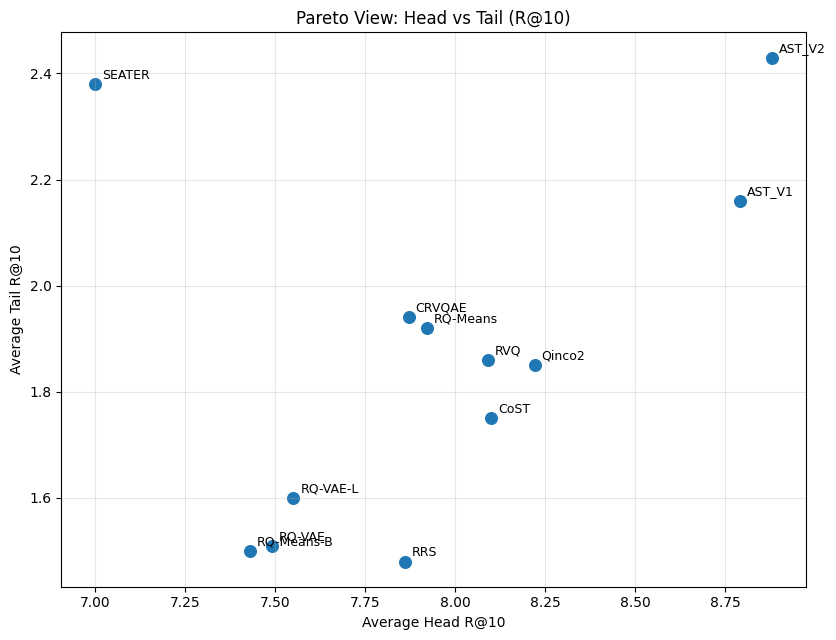
AST-V2 ranks first on average for head R@10 and head NDCG@10, first for tail R@10, and second for tail NDCG@10. Among the baselines, SEATER is strong on tail items and weak on head items, while RRS (which searches recursively over residual candidates until each item's SID is unique) leans toward head items. This shows that AST-V2's improvement does not trade one side for the other. In terms of the beauty store, both the best-selling matte lipsticks and the rarely bought hydrating lipsticks need to be recommendable, and AST-V2's average scores rank in the top two on both kinds of items.
How much do adaptive branching and the interaction requirement each contribute?
The authors test two simplifications. The first sets ρ to 0, removing the interaction requirement. The second removes adaptive branching so that every group uses one fixed branch count, tuned to its best value on each dataset, so the fixed-branching column below is already the best fixed branching can achieve.
| Dataset | Full AST (AST-V2) | Without interaction requirement | Fixed branching (tuned best) |
|---|---|---|---|
| Beauty | 7.51 | 7.33 | 7.01 |
| Toys | 7.94 | 7.73 | 7.36 |
| Sports | 4.62 | 4.54 | 4.56 |
| Health | 6.64 | 6.40 | 6.48 |
| Home | 3.02 | 2.98 | 2.95 |
All numbers in the table are R@10 (%). The full version is highest on all five datasets, which shows that both components help and that which one matters more varies by dataset. On Beauty and Toys, switching to fixed branching loses more; Beauty, for example, falls from 7.51 to 7.01. On Sports and Health, removing the interaction requirement loses more; Health, for example, falls from 6.64 to 6.40.
On Home, the largest dataset, both simplifications lose only a little, from 3.02 to 2.98 and 2.95. The authors' reading is that large datasets have many interactions, so every prefix on the tree already has enough training examples, while the interaction requirement and adaptive branching are more valuable when training examples are scarce, so the gap narrows.
Both simplified versions still exceed the strongest baselines in the earlier table on R@10; the fixed-branching version on Beauty has 7.01 against 6.98, and on Home 2.95 against 2.63. This shows that with either component removed, building SIDs as tree paths still leads on these datasets. The authors credit this to the basic structure of an SID as a tree path, but this ablation does not remove the tree itself, so it cannot isolate how much the tree structure alone contributes.
What needs tuning for a different catalog?
ρ needs tuning per dataset. The authors try ρ from 0.001 to 0.05; moderate values raise R@10 on some datasets and lower it on others. The authors explain that meeting the interaction requirement can put less similar items into the same branch, which lowers the similarity of items within a group. They also try SID lengths from 2 to 7; the best length is 4 for Beauty and 5 for the other four datasets, which shows that SID length, like ρ, should be chosen per dataset.
The choice of embedding has little effect on AST. Across three embedding models, M3, Qwen3 0.6B, and Qwen3 4B, AST's R@10 on Beauty only moves between 7.38 and 7.51. Under each embedding, AST is above the methods ranked second and third on that dataset in the main experiment. This shows that on these three embeddings its lead does not depend on any one of them.
When a new item launches, AST places it directly into the existing tree. Illustration: for a new woody perfume, AST computes its embedding and compares distances to the centers of the store's three groups, and the nearest is the perfume group; it then compares distances to the centers of the perfume group's two branches, and the nearest is the woody one. Each layer takes at most 4 comparisons, so two layers take at most 8, and the number of comparisons does not depend on how many items the store has. Placing the item in the tree only solves the coding problem, since the recommender has not been trained on this new SID, so cold start still has a gap on the model side.
The authors list two weaknesses of their own: SID quality depends on embedding quality, so noisy embeddings also hurt recommendations; and MILP may become computationally expensive at millions of items, at which point the authors say more efficient clustering and optimization methods are needed. All results come from 5 Amazon datasets, the largest of which, Home, has 28,237 items.
Back in the beauty store, AST changes only the table of SIDs: when the model writes the second token, "matte" has that meaning only after lip makeup, and the perfumes no longer have to be forced into 4 branches. When the tree is built to follow the order in which the model writes tokens, the same T5 averages about 13% above the strongest baseline on these five datasets.
How did this read for you?
Hoot made a note. Thanks for the feedback.

One tap, no sign-in; tap again to undo. Only anonymous counts are kept, never who you are.
Related papersMore from Paper Daily
 Generative · 2026-10-24GenPage: Towards End-to-End Generative Homepage Construction at NetflixThe Netflix homepage used to be assembled by a multi-stage recommender that retrieved candidate rows and titles, ranked them separately and then built the page; GenPage instead generates the whole page with one decoder-only Transformer. The homepage is made of rows, each row a theme. User history, account attributes and request information are encoded as a prompt, and the model generates row toke…
 Generative · 2026-11-05ReuseGR: Offline--Online Decoupled Generative Retrieval via Adaptive Prefix ReuseTeams putting generative retrieval into production should read this: it shows how to reuse large-model compute per query while leaving personalization to a small online model, and it is backed by an online A/B test. The same query is searched by many people every day, so generating a full Semantic ID from scratch for each request repeats work. ReuseGR splits the job in two. Offline, a large model…
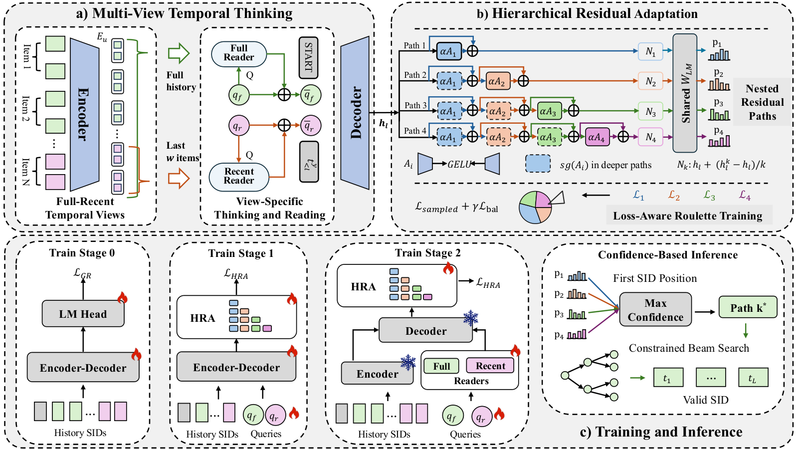 Generative · 2026-11-04Think Globally, Generate Personally: Multi-View Thinking with Adaptive Generation for Generative RecommendationIn SID generative recommendation, a user's newly emerging interest is often buried under a pile of old behavior, and every user shares one output transformation. This paper patches both weak spots in TIGER-style models. Before generation, the model gets two extra thinking tokens: one reads only the user's full history, the other reads only the last few items. The two resulting vectors sit at the…
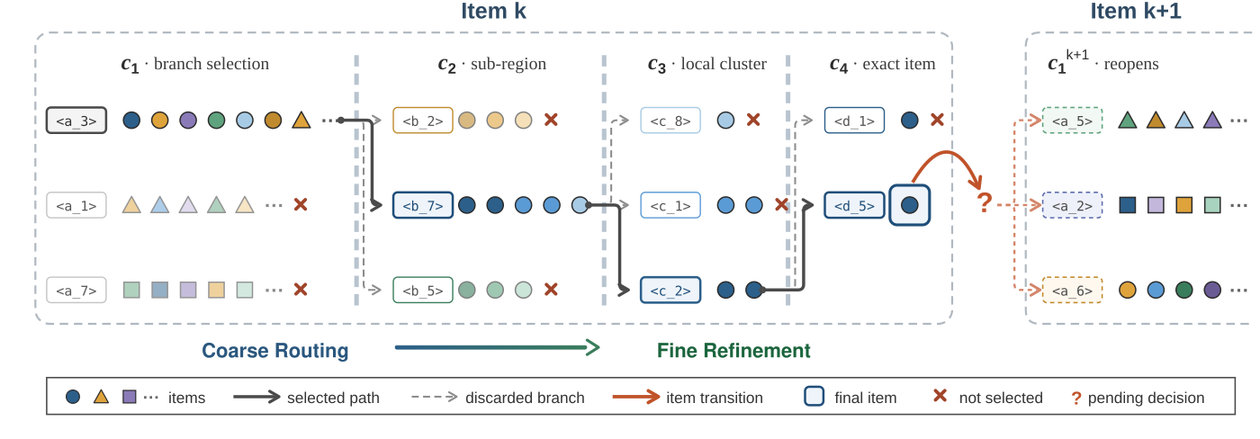 Generative · 2026-11-02RoFiGR: Coarse Routing, Fine Refinement via Level-Adaptive Distillation in Multimodal Generative RecommendationA generative recommender produces an item's SID one code at a time, and once the first two codes pick the wrong branch, no amount of later precision can recover the relevant items. In multimodal recommendation the SIDs are mostly built from image and text semantics, so their first codes may not reflect which items the same users tend to buy. RoFiGR therefore concentrates collaborative signal on t…
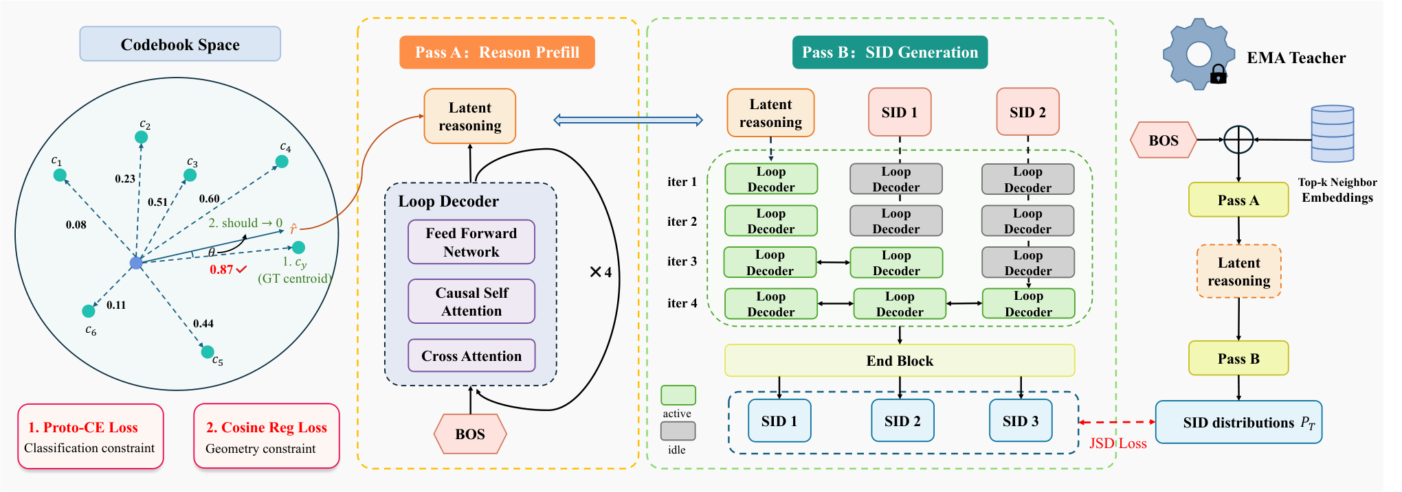 Generative · 2026-11-06BRIDGE: Bridging the Semantic Quantization Gap for Generative RecommendationGenerative retrieval predicts the next item's Semantic ID (SID) one code at a time from user history, but ordinary next-code training checks only the probability assigned to the correct code. When that probability stays the same, redistributing the remaining probability among incorrect candidates does not change this cross-entropy loss. BRIDGE (the generative retrieval model studied here) also us…
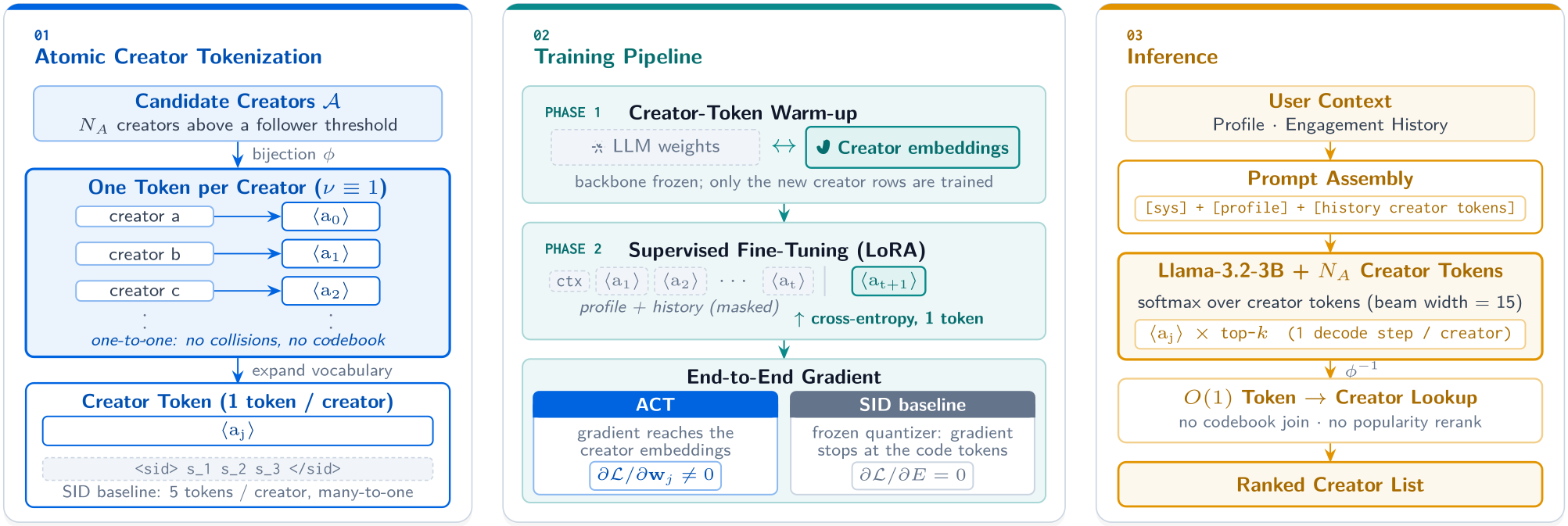 Generative · 2026-11-04Beyond Semantic IDs: Atomic Creator Tokens for Large-Scale Generative RecommendationThis Meta paper gives every creator its own token in the language model's vocabulary and uses it in place of the SID. The reason is simple: an SID is a many-to-one code, so several creators share one SID, and even when the model generates the right SID it still has to guess which of those creators the user wants. On Meta's creator recommendation data, swapping only the token layer lifts the share…
 Generative · 2026-11-04Utility-Aware Generative Recommendation: Utility-Enriched Semantic Codes and Utility-Guided DecodingThis Kuaishou paper adds video utility to two places in generative recommendation that used to look only at content and probability. 3 bits inside the last SID token record the video's utility tier: 7 ascending boundaries cut one utility statistic (such as historical click rate) into 8 tiers. At every beam-search step a small module reads the decoder hidden state, predicts behaviors such as watch…
 Generative · 2026-10-29REGER: Modeling inter-item Relations with Semantic IDs for Generative RecommendationCross-entropy tells a generative recommender only which token is correct, with no signal about how other candidates compare. REGER, from the University of Electronic Science and Technology of China, splits a conventional sequential model's scores over all items into branch preferences along the SID prefix tree and distills them along the true path. Added alone to TIGER, it lifts Beauty Recall@10…
Discussion
Add experiment details, reproduction notes or a different take. Requires a GitHub sign-in.
Loading the discussion…