Contents · 8 sections
1What problem is it solving?2How UAGR works: the big picture3How is the utility score computed during decoding?4How does utility get into the SID?5Experiments: does utility actually help?6Limitations as I see them7How a recommendation team could try it8VerdictSHARE

Teams building generative recommenders should read this. UAGR (the method proposed in this Kuaishou paper) adds video utility in two places that used to look only at content and probability: 3 bits inside the last SID token store a utility tier, and at every beam-search step a predicted utility score is added to the pruning score. There are two reasons for the change. Common generative recommenders build SIDs from content alone, so a video people usually finish and a video most people swipe away get nearly the same code whenever their content is similar. Beam search then prunes by generation probability alone, so a high-utility candidate can be cut at some middle token, and later reranking cannot bring it back. The utility score comes from the model's predictions of watch time, long view, like and share during decoding, added up with weights; SID length and vocabulary size stay the same.
It is fully deployed in Kuaishou's short-video recommendation; in a one-week A/B test video watch time rose 0.206%. Offline on KuaiRand, adding the decoding part alone lifts Recall@3 from 2.111% to 2.578%, above the 2.307% from reranking after generation and above the 2.418% from GRPO training on the same utility score. This means that utility used at the pruning step works better than utility used only for reranking after generation.
What problem is it solving?
A generative recommender encodes each video as a short SID, for example 3 tokens, each chosen from 8,192 codes. The model reads the user history, generates the SID one token at a time; the videos behind the generated SIDs are the recommendations. Generation uses beam search with beam width K.
The problem has two parts. First, SIDs come from clustering content embeddings, so similar videos get similar or even identical codes. Two videos that both show how to cook braised pork look the same in code, even if one is usually watched to the end and the other is mostly swiped away. Second, generation probability learns what appears in user histories; it does not directly reflect whether a user will finish, like or share a video after it is shown. When beam search drops a prefix by probability at a middle step, every video under that prefix is gone.
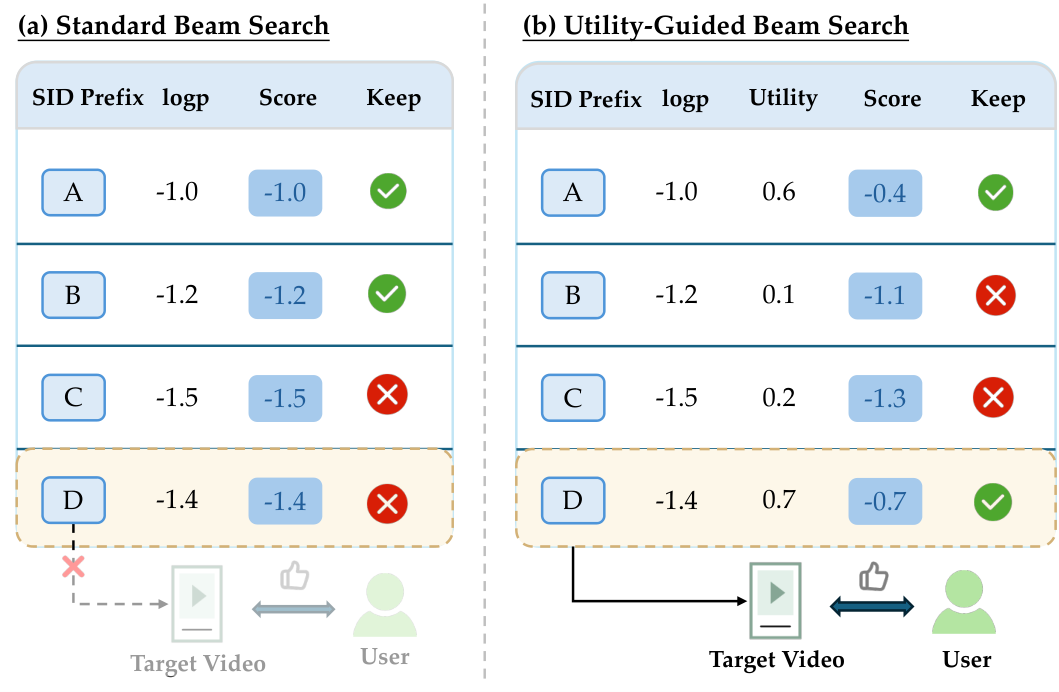
Figure 2 of the paper illustrates the second problem with four prefixes (the numbers are illustrative values from the paper's figure), with beam width K = 2:
| Prefix | Cumulative log-probability | Utility | Probability only | Probability plus utility |
|---|---|---|---|---|
| A | -1.0 | 0.6 | -1.0, kept | -0.4, kept |
| B | -1.2 | 0.1 | -1.2, kept | -1.1, dropped |
| C | -1.5 | 0.2 | -1.5, dropped | -1.3, dropped |
| D (the video the user would like is here) | -1.4 | 0.7 | -1.4, dropped | -0.7, kept |
By probability alone, D ranks third and is pruned, so the video the user would like can never be generated. After adding utility, D's total moves from -1.4 to -0.7, ranks second, and survives. Reranking after generation cannot do this, because it only reorders candidates that were already generated.
How UAGR works: the big picture
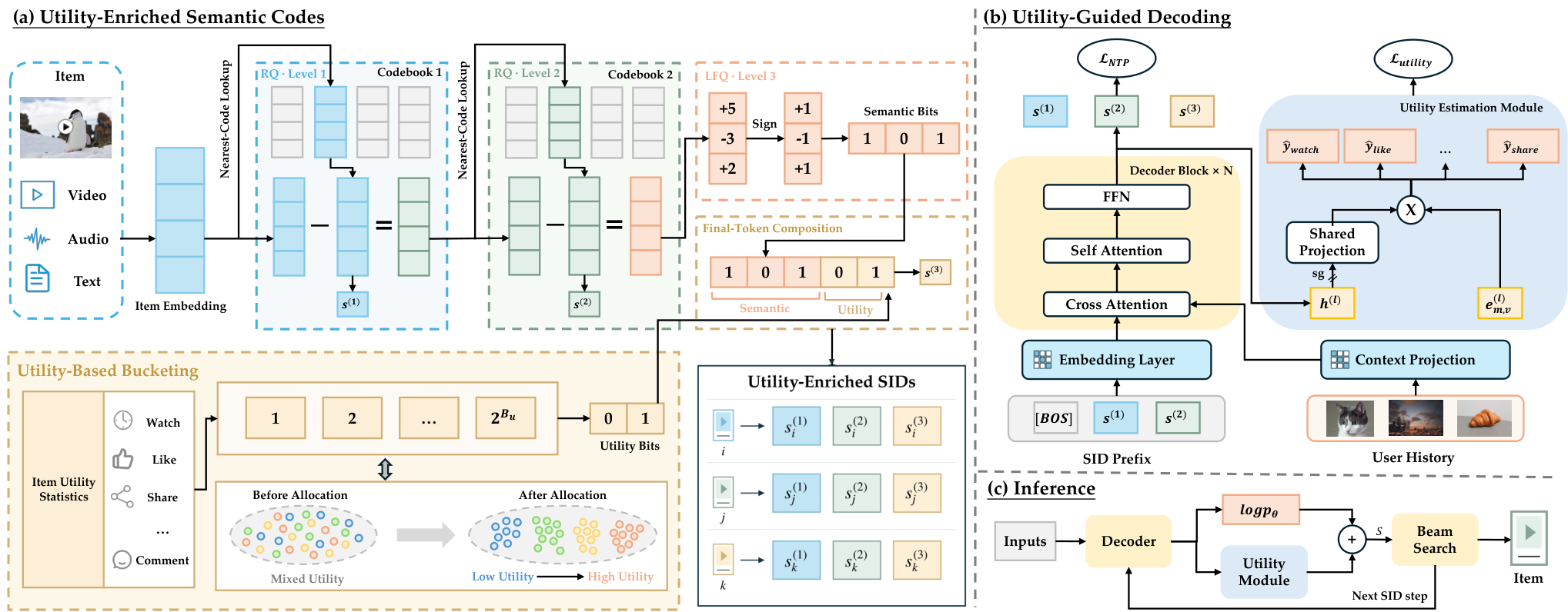
The method has two parts, each with one job:
| Part | When it acts | What it does |
|---|---|---|
| UGD | a small module added in training; used at every pruning step in inference | predicts post-exposure behaviors for each candidate token and adds a weighted utility score to the ranking |
| UE-SID | when SIDs are built | reserves 3 bits in the last token for a utility tier, so videos with similar content but different utility get different codes |
The code side makes videos with different utility separable in SID space; the decoding side makes utility count at pruning time. The sections below take them in turn.
How is the utility score computed during decoding?
The paper calls this part UGD (short for Utility-Guided Decoding). It is needed because beam search decides what to keep at every step, and probability only reflects relevance. To consider utility during pruning, there must be a utility estimate at every step for every candidate token.
The utility module reuses the generator's own computation. At position l, the decoder has already produced a hidden state from the user history and the generated prefix. A small MLP compresses that hidden state into a low-dimensional vector shared by four behaviors. Each behavior then has a learnable vector and bias for each candidate token (a separate set at each token position); their inner product with the shared vector gives the predicted score for that behavior if this token is appended. The four behaviors are watch time, long view, like and share.
At pruning time, each candidate's total score is:
The first term is the cumulative log-probability so far. is behavior m's predicted score for candidate token v. Norm puts the behaviors on one scale: binary predictions such as like go through a sigmoid; regression predictions such as watch time are standardized across the current step's candidates and then go through a sigmoid. are the behavior weights, set to 0.6 for watch time, 0.2 for long view, 0.1 for like and 0.1 for share, with = 1.
One detail is easy to miss: probability accumulates over tokens, but utility does not. The ranking score is the cumulative log-probability plus the utility score of the current step's candidate token; utility from earlier steps is not carried in. Hoot says

- Utility (illustrative): 0.6 × 0.9 + 0.2 × 0.5 + 0.1 × 0.2 + 0.1 × 0 = 0.66
- Score (illustrative): cumulative log-prob −1.4 plus 1 × 0.66 gives −0.74; it only decides whether the prefix is kept
- What enters the next step is still −1.4 plus the next token's log-prob; this step's 0.66 is not carried, so a long prefix does not add utility several times over.
Illustrative: one candidate token for one prefix at one step. The left column is what this step computes; the right column is pruning and the next step. The normalized behavior predictions are made up; the weights 0.6, 0.2, 0.1, 0.1 and λ = 1 are the paper's settings. Source: paper §3.2 ranking score (cumulative log-probability + λ·weighted normalized predictions, utility from the current step only), utility heads reading stop-gradient decoder hidden states; Appendix B.2 weights and λ
At inference the module reads only the hidden state and never sees real feedback. Real feedback appears only in training: each training sample is a user history plus a target video, and the recorded outcomes of that video after exposure (long view or not, how long it was watched, like, share) are labels that supervise the module's predictions at every token of the target SID. In the offline experiments these labels come from all training-period exposures, including exposures without a long view, and never from validation or test data. The training objective is the usual next-token loss plus a utility loss with weight 0.001.
A stop-gradient sits where the module reads the decoder hidden state. The generator is still trained as usual with the next-token loss (LoRA fine-tuning in the paper), just without interference from noisy behavior labels. Adding a new behavior later only needs a new head. At inference these heads run in the same forward pass as next-token prediction, so no extra pass of the model is needed.
How does utility get into the SID?
If two videos share exactly the same SID, decoding cannot tell them apart, however good the utility score is. The paper calls this an SID collision. With the usual three-level residual K-means on KuaiRand, 4.29% of videos collide with another video on the same SID.
The paper's code design, UE-SID (short for Utility-Enriched SID), changes only the last token; the first two stay residual K-means. The last token's 8,192 codes are exactly 13 bits. It works in three steps:
- Turn the last token into 13 independent 0/1 bits. A learnable linear projection maps the residual left after the first two levels into 13 numbers, and each number becomes 1 if positive and 0 otherwise. This is called LFQ (lookup-free quantization: bits are read off signs instead of looking up a codebook). The projection is trained with two terms. One pulls each of the 13 numbers toward the +1 or −1 it snaps to, so little is lost when bits are taken. The other is an entropy regularizer that keeps all codes in use, so videos do not pile onto a few codes. The paper adds no reconstruction loss; the content in the bits comes from the input itself, which is the content residual the first two levels left over.
- Free the 3 least useful bits. There are 286 ways to choose 3 of 13 bits; the authors try them all and pick the 3 whose removal raises collisions the least.
- Store a utility tier in the freed 3 bits. Three bits can hold exactly 8 tiers, so seven ascending boundary values cut the utility statistic into 8 tiers, numbered 0 to 7. A video's tier is the number of boundaries its statistic reaches, and that index is written into those bits. In the offline experiments the statistic is the video's historical click-through rate.
An example (illustrative): two braised-pork videos have identical 10 content bits, 1011001110; one has a click-through rate in tier number 6, written 110, the other in tier number 1, written 001. Concatenated they become two different codes, so the model can generate them separately. The code count is still 8,192 and the vocabulary does not change.
Experiments: does utility actually help?
Offline experiments use KuaiRand-27K, a public Kuaishou short-video dataset with several kinds of post-exposure feedback. Each user's positive sequence keeps only long-view videos, and the last one is held out for testing. The generator is OneRec-1.7B fine-tuned with LoRA, with beam width 200. All rows of the table below share the same base model.
| Method (KuaiRand) | Recall@3 | NDCG@3 | Recall@5 | NDCG@5 |
|---|---|---|---|---|
| Base model | 2.111 | 1.643 | 3.149 | 2.046 |
| + post-generation reranking | 2.307 | 1.675 | 3.275 | 2.083 |
| + GRPO training | 2.418 | 1.953 | 3.602 | 2.450 |
| + UE-SID only | 2.409 | 1.967 | 3.585 | 2.436 |
| + UGD only | 2.578 | 2.047 | 3.712 | 2.499 |
| Full UAGR | 2.774 | 2.274 | 3.963 | 2.776 |
(in %, from Table 3 of the paper)
First, what decoding should be compared against. Reranking and GRPO use the same utility score with the same four weights; only where it is used differs. Reranking reorders after generation, and GRPO uses the score as a training reward. UGD alone beats reranking by 0.27 points of Recall@3 and GRPO by 0.16 points. The same utility signal is worth more at pruning time than after generation or during training. GRPO optimizes a reward on complete SIDs; it changes generation probabilities and so affects pruning indirectly, but it does not guarantee that high-utility prefixes survive the middle pruning steps. UGD changes the pruning score at every step directly.
Against other kinds of methods, full UAGR is the best of all methods in Table 1 of the paper, 7.74% above the strongest baseline in Recall@3. Single parts are roughly on par with strong existing baselines: UGD alone at 2.578 is almost the same as RecForest at 2.575. The gain of any single part should not be overrated; the two parts together open the gap.
Next, the codes. UE-SID alone lifts Recall@3 from 2.111 to 2.409. The appendix breakdown shows each step's role: switching to 13-bit LFQ alone makes videos easier to tell apart and improves recommendation; dropping the 3 weakest bits makes recommendation slightly better still; adding 3 utility bits then lifts every recommendation metric clearly. The authors also tried learning a 10-bit LFQ directly plus the same 3 utility bits: the code capacity is identical, but Recall@3 is only 2.168. The authors' explanation is that learning only 10 bits from the start squeezes too hard and loses content distinctions useful for recommendation, while learning 13 and dropping the weakest 3 keeps more of them. This is one comparison on one dataset.
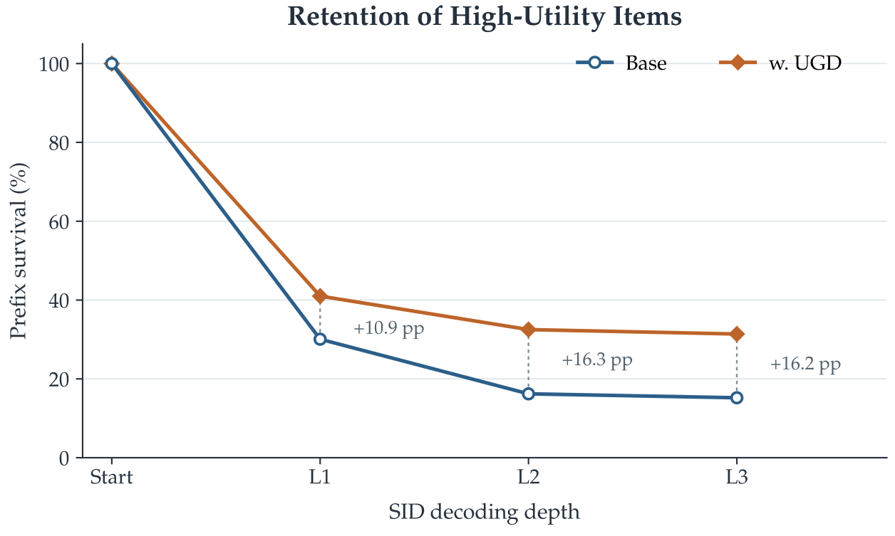
The most direct evidence is Figure 3. The authors treat videos with long-view feedback as high-utility videos, take the set present before decoding starts as the denominator, and count how many of their prefixes are still in the beam after each decoded token. This is an evaluation-time count: the long-view labels only pick out this set, and during decoding the model uses only its own predictions. At the same beam width, UGD keeps 10.9 percentage points more after the first token, the gap is largest after the second token at 16.3 points, and it stays at 16.2 points after the third (values read from the figure's annotations). Utility helps from the first pruning step, and the gap is widest at the middle token.
Online, UAGR replaced the production generator in Kuaishou short-video recommendation for a one-week A/B test: app usage time +0.074%, video watch time +0.206%, video views +0.164%, all significant at p<0.05, with QPS down only 0.03%. The cost of a few extra heads per step is negligible in serving. UAGR has been fully deployed on Kuaishou since September 2026.
Limitations as I see them
First, offline metrics are very low in absolute terms. Recall@3 is around 2%, and full UAGR is 0.66 points above the base model. There is only one dataset, KuaiRand-27K, with no replication on other data or other base models.
Second, online results are reported only as a whole. The 0.206% watch-time gain comes from UGD and UE-SID together, with no separate online test, so we cannot tell which part drives the online gain.
Third, the four utility weights and are one hand-set choice: watch time 0.6, long view 0.2, like 0.1, share 0.1, with = 1. All results use this one setting. A different business goal needs new weights, and the current experiments cannot show how sensitive the results are to them.
How a recommendation team could try it
- Start with the decoding utility score only. In the paper the behavior heads train jointly with the generator, separated by stop-gradient; for a cheaper start you can freeze your existing generator and train only a few heads on its hidden states, which is my simplification. Add the weighted utility score to the cumulative probability when pruning. As a control, use the same score for post-generation reranking, to check that the gain comes from the pruning step.
- Track per-position prefix retention of high-utility targets, as in Figure 3. If retention does not rise clearly at any token, the utility score is not doing its job; see step 4 for tuning.
- Then measure the collision rate of your current SIDs. If it is several percent or more, try switching the last token to bit codes and freeing a few bits for a utility tier.
- Treat the four weights and as hyperparameters to tune: sweep a few settings offline, then A/B test one or two online, since the paper reports a single setting.
Verdict
In generative recommendation, utility signals matter most at the moment beam search prunes; reserving a few code bits for utility lets videos with similar content be told apart.
| Dimension | Assessment |
|---|---|
| Problem importance | High. Candidates pruned at a middle prefix cannot be rescued by later reranking, and sequence-level rewards only affect pruning indirectly |
| Novelty | Medium. Adding a per-step utility score and reserving code bits are simple, but the two fit together well and the current-step-only scoring is clean |
| Evidence | Medium. Same-condition comparisons with reranking and GRPO plus per-position retention analysis, but only one offline dataset and no online split by component |
| Engineering cost | Low to medium. A few light heads and no extra forward pass at inference; codes need a rebuilt last token |
| Worth trying | Yes. Teams already running generative retrieval with several kinds of post-exposure feedback can start with the decoding utility score |
How did this read for you?
Hoot made a note. Thanks for the feedback.

One tap, no sign-in; tap again to undo. Only anonymous counts are kept, never who you are.
Related papersMore from Paper Daily
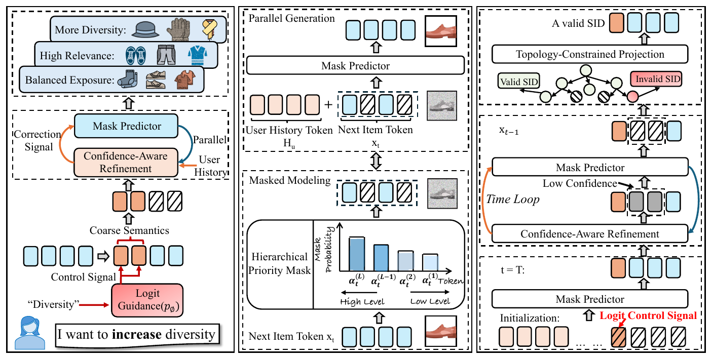 Generative · 2026-10-23Controllable Generative Recommendation via Guided Token RefinementGenerative recommenders emit item-ID tokens left to right, so temporary diversity at inference can only rewrite one position mid-decode and often produces IDs that do not exist in the catalog. ReGen uses a bidirectional Transformer to predict all 4 ID tokens at once, subtracts a score only on the coarsest positions for token values common in the user history, remasks low-confidence positions and…
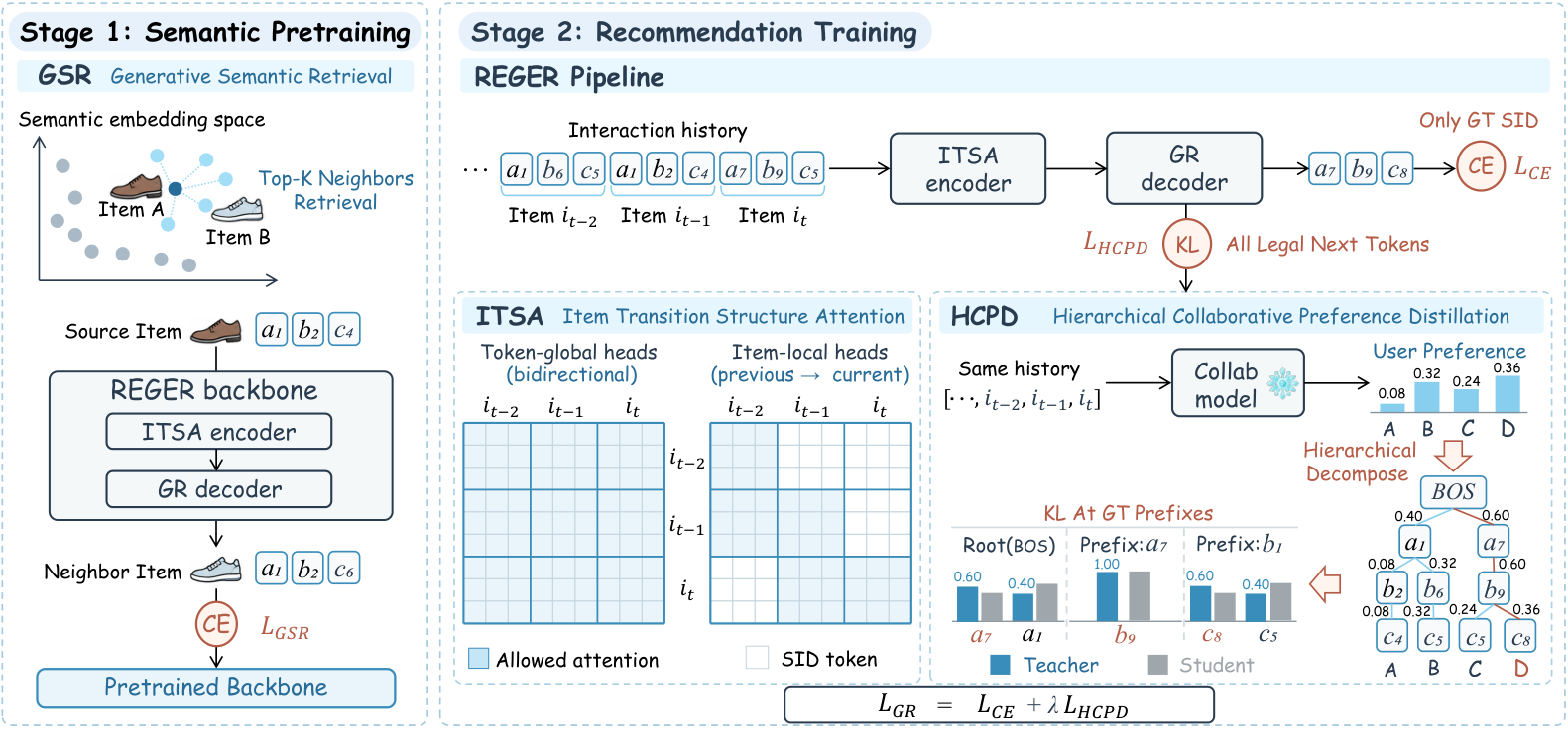 Generative · 2026-10-29REGER: Modeling inter-item Relations with Semantic IDs for Generative RecommendationCross-entropy tells a generative recommender only which token is correct, with no signal about how other candidates compare. REGER, from the University of Electronic Science and Technology of China, splits a conventional sequential model's scores over all items into branch preferences along the SID prefix tree and distills them along the true path. Added alone to TIGER, it lifts Beauty Recall@10…
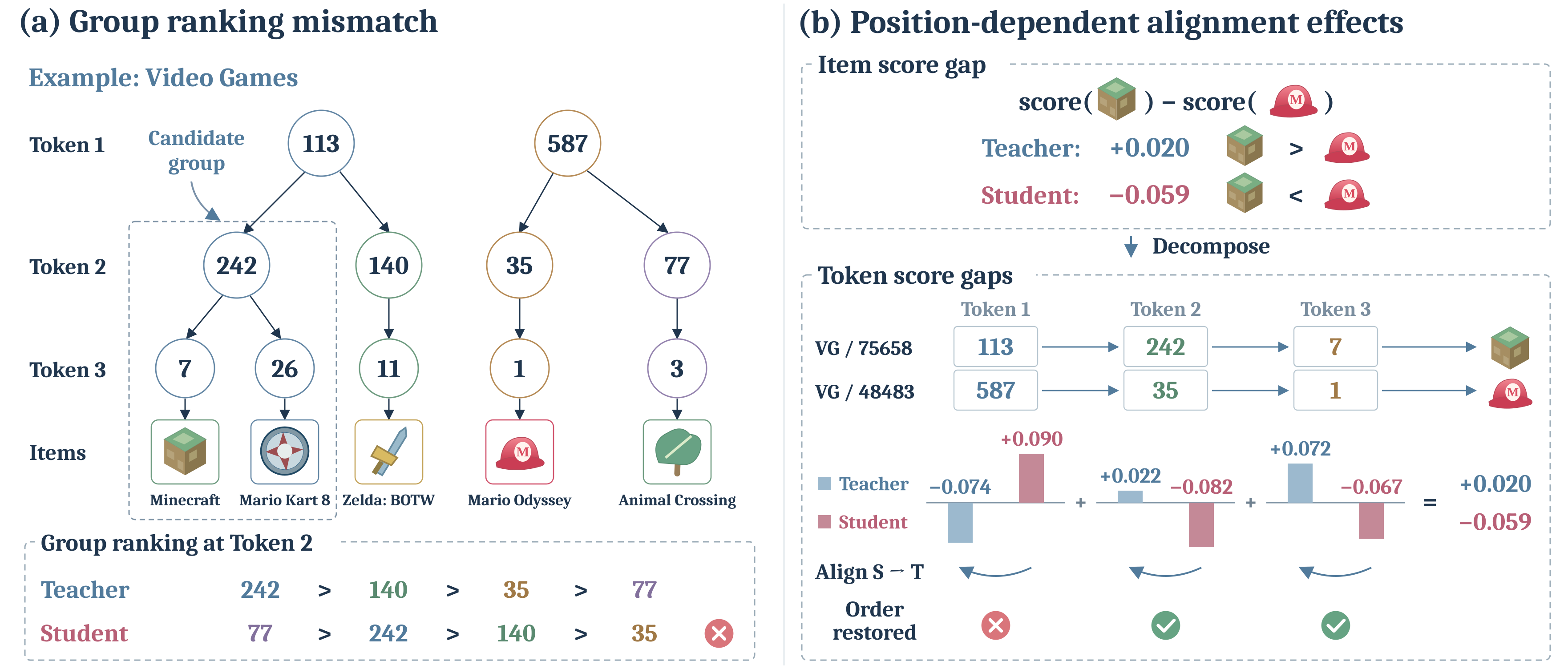 Generative · 2026-10-28MuSID-KD: Multigranularity Knowledge Distillation for Generative Recommendation with Semantic IDsWhen a SID-based generative recommender is distilled into a small model, the student is usually asked only to match the teacher's distribution over which item to recommend in the end. ECNU's MuSID-KD (a multi-granularity distillation method that works level by level over the SID) finds this is not enough: a student aligned only on items disagrees with the teacher on the order of candidate groups…
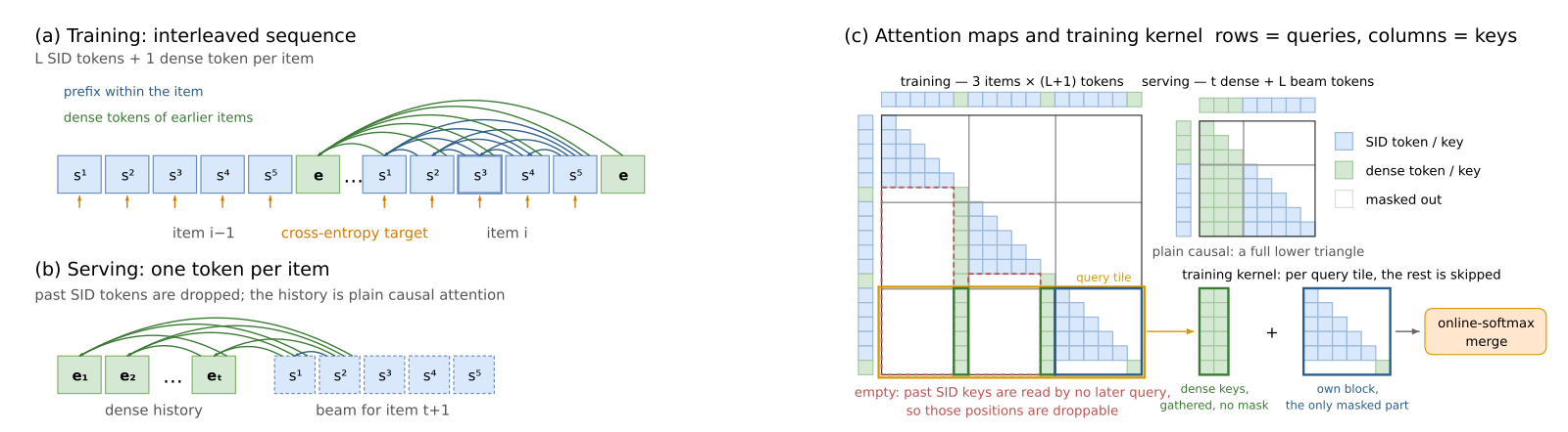 Generative · 2026-10-28PinGER: Token-Efficient Generative Retrieval with Semantic IDsGenerative retrieval encodes each item as a multi-level SID and generates it level by level, but on the input side every history item costs several tokens. During training, Pinterest's PinGER places one dense-vector token after each item's SID and requires that any token reading another item may see only that item's dense token, never its SID. At serving time all SIDs in the history can be droppe…
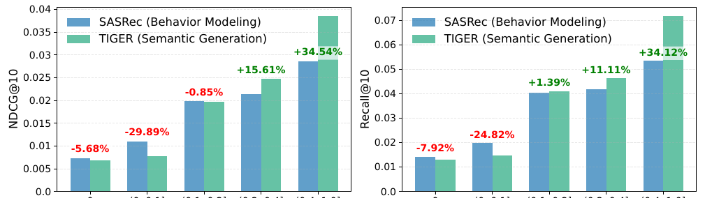 Generative · 2026-10-27Unifying Behavior Modeling and Semantic Generation for Generative RecommendationGenerative recommenders that write the next item's Semantic ID code by code have a systematic bias. This KDD 2026 paper from South China University of Technology finds that the fewer items in a user's history share the target's category, the worse they do against classic behavior-only sequential models; in the worst group, TIGER's NDCG@10 trails SASRec by 30%. The cause: the encoder learns which…
 Generative · 2026-10-26From Item Scores to Semantic Tokens: Test-Time Collaborative Adaptation for Generative RecommendationIn generative recommendation with semantic IDs, the model writes an item's code one token at a time, and beam search keeps only the highest-scoring prefixes at each step. Once a prefix is pruned, every item beneath it can never be generated. The problem is sharpest when a user has just developed a new interest that shows up in only one or two recent interactions. This paper proposes TCBSA (test-t…
 Generative · 2026-10-22Evolving Semantic Indexes for Generative RetrievalAn LLM evolves executable semantic-index programs while a tiny retriever screens them. With the target training recipe fixed, NQ320K Recall@100 rises from 85.82% to 90.57%.
Discussion
Add experiment details, reproduction notes or a different take. Requires a GitHub sign-in.
Loading the discussion…