Contents · 9 sections
1What problem is it actually solving?2The overall flow: cluster first, then draw negatives from the same cluster3Why are negatives from the same cluster more useful?4Where do the clusters come from, and why LLM content vectors?5The real-time item pool: how do you draw by cluster in streaming training?6What do the results show?7Where I think it falls short8How a recommendation team could try it9VerdictSHARE

Teams that run two-tower retrieval should read this one. It tackles an old problem that industrial systems still handle poorly: the negatives used to train a two-tower model are too easy, so the model soon stops learning from them. Existing hard-negative methods either score the whole corpus or maintain a global nearest-neighbor index, which is too expensive for large-scale streaming training. The core idea in one sentence: group items into a few hundred content clusters, draw negatives at random from the same cluster as the positive item, and make this real-time with an in-memory item pool that is split into one segment per cluster. The paper comes from Meta and appeared at the RecSys 2026 workshop on online and adaptive recommender systems. In a social app with about one hundred million monthly users, this retrieval source's CTR rose 53% and system-wide CTR rose 6.5%, while training throughput fell only 1.4%. The share of impressions taken by the top 100 items dropped from 50% to 32%. On public data, HR@50 on Amazon-Electronics went from 0.0084 to 0.0131.
What problem is it actually solving?
Start with an illustrative scenario. A user on a content-discovery page opens a post about camping gear, and that click is a positive. When training the two-tower model, we want this user's embedding to sit close to that post and far from other posts. The question is where the "other posts" come from.
| Negative source (illustrative) | Posts drawn | Similarity to the camping post | What the model learns |
|---|---|---|---|
| Other users' clicked posts in the same batch | A cat video, a football highlight | Very low | Almost nothing; they were already easy to separate |
| Random draw from the whole corpus | A recipe, a phone review | Very low | Same as above |
| Random draw from the same content cluster | Another tent review, a hiking route | Fairly high | Which kind of camping content this user prefers |
The first two rows are the most common industry practice. In-batch negative sampling costs almost no extra compute, but the range of negatives is capped by the batch size. Out-of-batch (OOB below) sampling covers more items, and the candidates seen in training are closer to the full corpus the model faces online. But items drawn at random from the whole corpus mostly have nothing to do with the user's interests. The paper's view is that random OOB negatives are too easy for the model, and the larger and more diverse the pool, the worse this gets.
Existing hard-negative methods do find negatives that look more like the positive. DNS (Dynamic Negative Sampling) scores candidates with the current model and picks the highest-scoring items the user did not click. ANCE builds an approximate nearest-neighbor index over the whole corpus, refreshes it asynchronously during training, and takes the items closest to the query as negatives. One method must score many candidates at every step and the other must keep rebuilding a corpus-wide index. The paper argues this cost is why such methods have not spread to large industrial systems.
A second problem is tied to negatives: popularity bias. Retrieval models use clicks as positives, and what a user can click depends on what the system showed them. Popular items get more impressions, more clicks and more turns as positives, so the next round pushes them even harder. In the paper's production app there are tens of millions of eligible posts, yet the top 100 items take about half of all impressions.
The overall flow: cluster first, then draw negatives from the same cluster
The scheme has an offline part and a training-time part. This table gives the overview.
| Part | When | Input | Output |
|---|---|---|---|
| Content embedding | Offline, when an item enters the corpus | The item's text, images, audio and video | One fixed-length content vector per item |
| Clustering | Offline k-means; new items go to the nearest centroid as they arrive | Content vectors | One cluster ID per item |
| Pool update | During training, every batch | IDs, cluster IDs and features of the items in the batch | The matching pool positions overwritten with the newest items |
| In-cluster sampling | During training, every batch | Cluster IDs of the positives in the batch | Negatives taken at random from positions of the same cluster |
| Training | During training | Positives, in-batch negatives, random OOB negatives, same-cluster negatives | Updated two-tower parameters |
The key division of labor is that the content model only groups items; it never enters the online retrieval path. Serving is still the original two-tower model plus nearest-neighbor search, so inference throughput does not change.
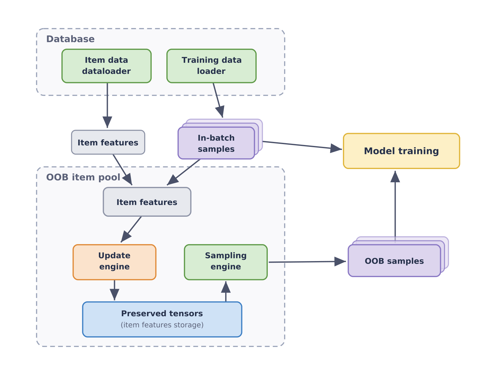
The paper calls the version that ignores clusters and samples the pool uniformly GOOBS (Global Out-of-Batch Sampling). The version that adds same-cluster negatives is Cluster GOOBS. The parts are covered one by one below.
Why are negatives from the same cluster more useful?
Two-tower training usually treats retrieval as a very large multi-class problem: given a user, predict which item among all items they clicked. A softmax over the whole corpus is too expensive, so it is computed only over the positive and K sampled negatives:
Here is the user, is the item they clicked, is the k-th negative, and is the inner product of the user-tower and item-tower outputs. The intuition: the numerator should be large and the negative terms in the denominator should be small.
The paper explains the method through gradients. A negative's gradient with respect to the user vector is proportional to . Take an example you can work by hand (illustrative): the positive scores 5. A random negative lies far from the user and scores 0; a same-cluster negative has similar content and scores 4.
- With only the random negative, its softmax share is .
- With only the same-cluster negative, its share is .
This share is exactly the derivative of the loss with respect to that negative's score, so at the score level the same-cluster negative receives an update signal nearly 40 times larger. On the user vector it is further multiplied by the negative's own item vector, but the difference in magnitude comes mainly from this share. The random negative's gradient is close to zero: the training step is spent, yet the model barely moves. The same-cluster negative sits near the model's current decision boundary. It forces the model to learn fine differences within one kind of content, rather than a distinction like "camping is not a cat video" that it learned long ago. The paper notes this matches ANCE's theoretical finding that negatives closer to the query carry larger gradients.
The same analysis predicts a pitfall. Because same-cluster negatives carry large gradients, giving each positive too many of them lets that part of the loss dominate and destabilizes training. The paper varied the number of same-cluster negatives per positive from 1 to 64 and found that a small number works best, while larger counts hurt. In the public experiments the ratio of same-cluster to random OOB negatives is 1:15 on MovieLens-1M and 1:31 on Amazon, so most negatives are still random and only a small share come from the cluster.
Where do the clusters come from, and why LLM content vectors?
Cluster quality decides whether same-cluster negatives are really "similar". The traditional choice is category or genre. The paper's production deployment instead uses an in-house multimodal content-embedding model: encoders for text, images, audio and video built on a pre-trained LLM encode each item into a fixed-length vector, and the model is then fine-tuned for the target task.
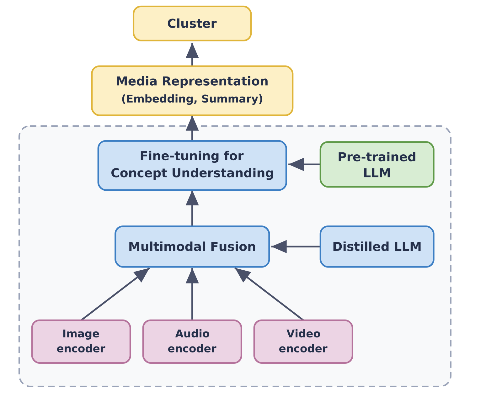
Given the vectors, k-means forms the clusters. Each item goes to its nearest centroid, and new items are assigned online once encoded. Items in one cluster are then genuinely close in content, not merely filed under the same category.
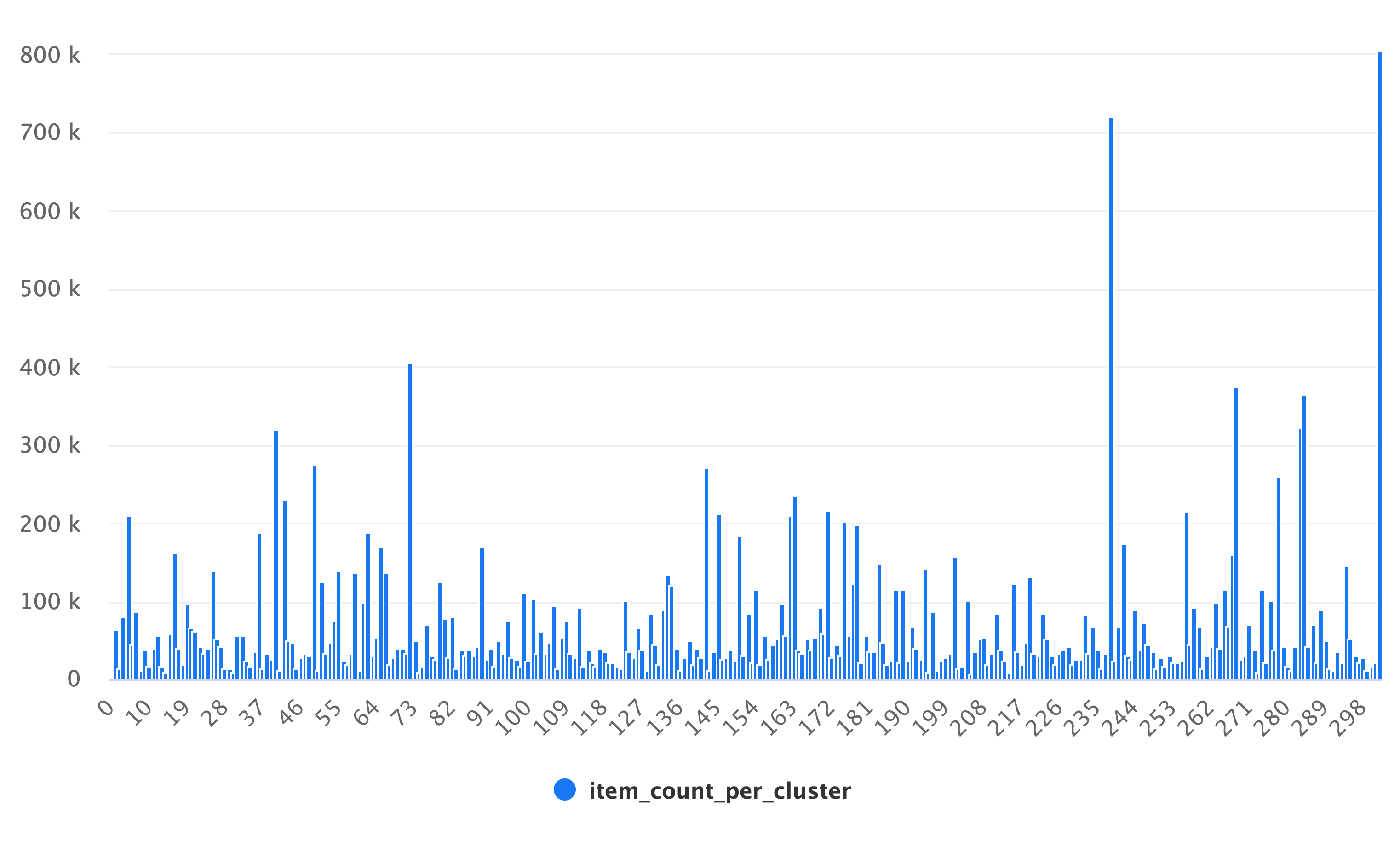
The number of clusters is a trade-off. If clusters are too fine, items in the cluster are almost the same as the positive, and the user may well like them too, so drawing them as negatives creates false negatives. If clusters are too coarse, items in the cluster are not similar enough and the negatives are not hard enough. An offline sweep from 100 to 10,000 clusters found 250 to 500 the best balance, so production uses 300 clusters. With that split, 98% of clusters hold at least ten thousand items, which shows the clusters are not fine and the false-negative risk stays under control.
Why not worry much about false negatives? The paper gives an estimate: a user is genuinely interested in at most a few thousand items out of billions, and a cluster holds about ten thousand items, so the share truly relevant to one user is well below 1%. Because each step samples at random, the rare relevant item that does get drawn is also spread over different training steps. This is the paper's estimate, not a measured false-negative rate.
The real-time item pool: how do you draw by cluster in streaming training?
Cluster IDs alone are not enough. Training data keeps flowing in, the item pool has to keep up, and sampling must not slow training down. The paper keeps a fixed-size item pool in memory, split by cluster.
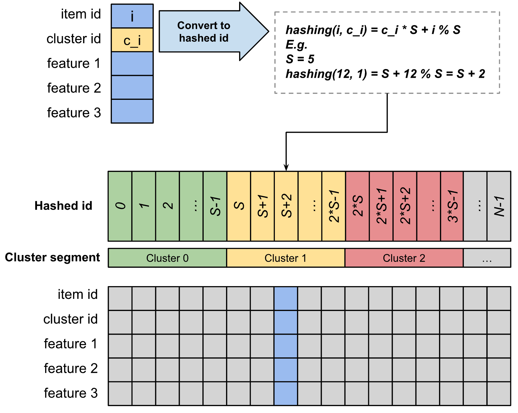
The pool consists of many positions (the paper calls them slots), and each position stores all the features of one item. The pool is cut into segments, one per cluster, each with the same number of positions, written S. "Draw an item from a given cluster" then becomes "pick a random position in one segment", with no index needed.
Writing works like this. For each training batch and each item in it, look up its cluster ID c and compute a position:
A hand-worked example (illustrative): with 4 positions per segment, an item with ID 1234 in cluster 7 is written to position . When two items map to the same position, the later one simply overwrites the earlier one. The paper says this is by design: the pool keeps getting refreshed with recently seen items, and its memory footprint stays fixed.
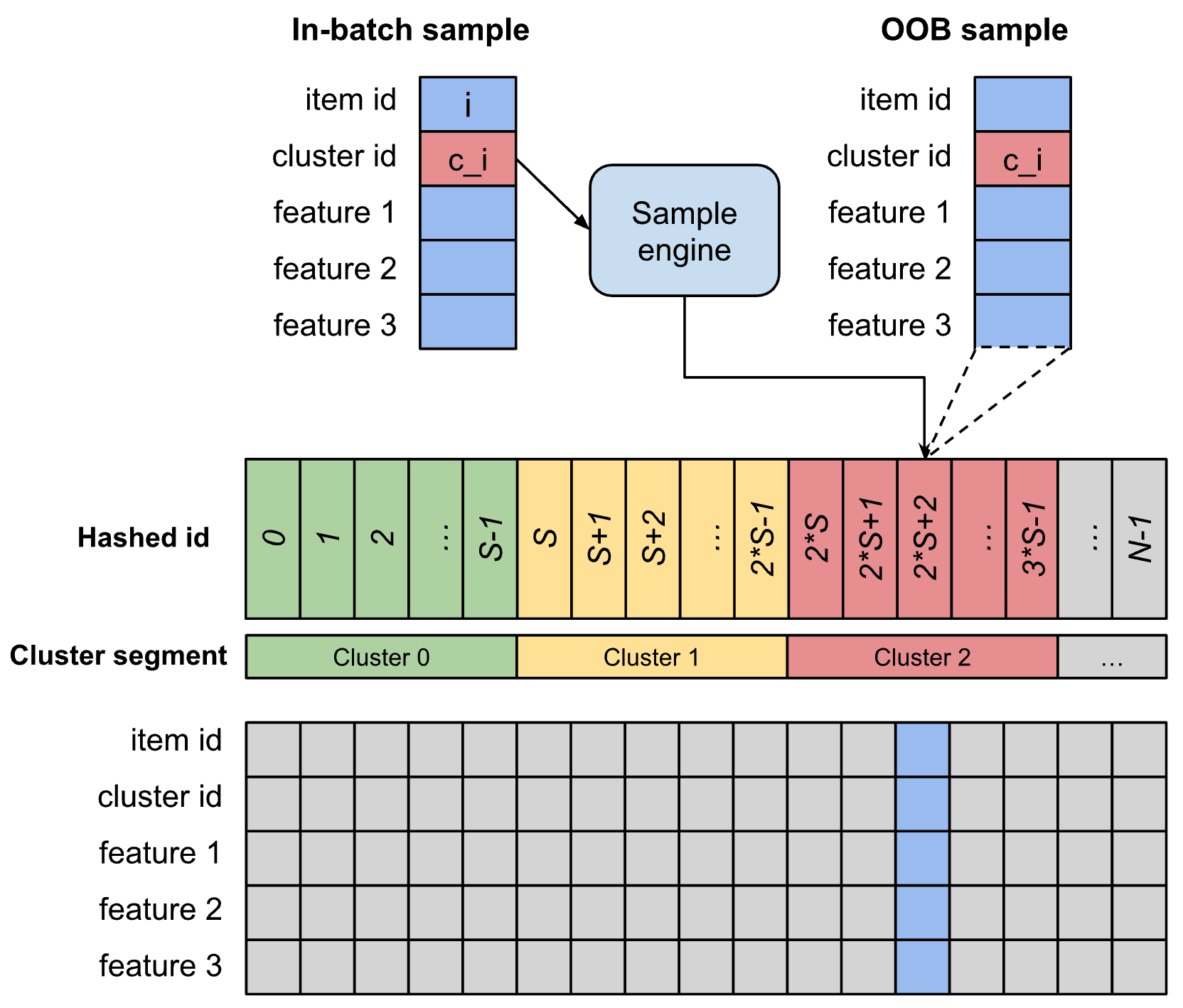
Sampling is just as simple. For each positive in the batch, take its cluster ID c, draw a random number r between 0 and S, and take the item at position as a negative. Continuing the example, a positive in cluster 7 that draws r=1 takes the item at position 29. Following the loss in Section 3.2 of the paper, each positive's denominator holds the few negatives it drew itself, plus in-batch and random OOB negatives. How exactly these negatives are combined with the in-batch samples into one computation is described only as far as "combined with in-batch samples for training".
At the start of training the pool is empty, and drawing by cluster would often come up with nothing. The paper pre-loads the pool before training with an item table built from earlier training data. That data is a bit older than the latest training data, but as training proceeds new items from each batch keep overwriting it, so the pool stays fresh.
Why is this design cheap? Writing and sampling only look up a cluster ID, compute an index and read or write a block of memory. Nothing scores candidates and no nearest-neighbor index is rebuilt. In the online experiment, training throughput fell only 1.4%.
What do the results show?
Public datasets
This experiment asks whether, on the same two-tower model with only the negative sampler changed, in-cluster sampling beats existing methods. The datasets are MovieLens-1M and the Grocery, Electronics and Home subsets of Amazon Reviews. Data is sorted by time: the first 80% is for training and the last 20% for testing. Ratings 1–2 are negatives and 3–5 are positives. At evaluation the target item is ranked against every item in the corpus. There is no k-core filtering, and ranking is not limited to 100 random negatives. Absolute numbers are therefore low, but closer to real sparse settings.
One point first: the clusters on public data are the categories or genres shipped with the datasets, not LLM clusters. The paper's reason is that these datasets hold only tens to hundreds of thousands of items, each with a title and a few attributes, so LLM clustering would mostly recover the existing categories. The authors say plainly that they make no claim that LLM clusters beat categories on public data. This experiment therefore tests the mechanism of "draw negatives from the same cluster" itself.
All six methods are built on the same two-tower model. The baseline is in-batch sampling with LogQ correction, and it masks in-batch negatives that are actually known positives. The others are DNS, CBNS (Cross-Batch Negative Sampling, which caches item embeddings from recent batches and reuses them as negatives), ANCE, GOOBS and Cluster GOOBS.
| Dataset | Metric | Baseline | DNS | CBNS | ANCE | GOOBS | Cluster GOOBS |
|---|---|---|---|---|---|---|---|
| MovieLens-1M | HR@50 | 0.2253 | 0.2298 | 0.2331 | 0.2380 | 0.2346 | 0.2415 (+7.2%) |
| MovieLens-1M | HR@100 | 0.3588 | 0.3618 | 0.3608 | 0.3661 | 0.3611 | 0.3682 (+2.7%) |
| Amazon-Grocery | HR@50 | 0.0254 | 0.0261 | 0.0271 | 0.0288 | 0.0279 | 0.0301 (+18.5%) |
| Amazon-Electronics | HR@50 | 0.0084 | 0.0090 | 0.0099 | 0.0108 | 0.0110 | 0.0131 (+55.6%) |
| Amazon-Electronics | HR@100 | 0.0154 | 0.0163 | 0.0176 | 0.0186 | 0.0190 | 0.0201 (+30.2%) |
| Amazon-Home | HR@50 | 0.0050 | 0.0054 | 0.0061 | 0.0065 | 0.0067 | 0.0074 (+47.3%) |
(Numbers from the paper's Table 1; parentheses show the gain over the baseline. The HR@100 rows for Grocery and Home are left out; Cluster GOOBS is best there too, at +15.7% and +42.3%.)
Three things can be read from this table.
First, just widening negatives beyond the batch already helps. GOOBS picks no hard negatives at all, yet its HR@50 gain over the baseline ranges from 4.2% to 34.2%. This shows that seeing a wider range of items in training by itself makes the model generalize better.
Second, adding a few same-cluster negatives on top of random OOB is best on every dataset and every metric, including ANCE, which needs a global nearest-neighbor index. The gap is largest on the sparse Amazon data: on Electronics, Cluster GOOBS lifts HR@50 by 55.6% against 28.6% for ANCE. This suggests that on data with many items and sparse interactions, negatives grouped by content work better than neighbors found with the current model's vectors.
Third, gains on HR@50 are generally larger than on HR@100. The paper takes this to mean that same-cluster negatives mainly help the model put the most relevant items at the very top of the retrieved list, which is the part later ranking stages depend on most.
Online A/B test
The online test asks whether the effect holds with LLM clusters on real traffic. The app is the content-discovery entry of a social app with about one hundred million monthly users. It has tens of millions of eligible posts, and the model trains on billions of interactions. Control and test each get a random 3% of users for 14 days. Both use the same two-tower architecture: control uses GOOBS and test uses Cluster GOOBS. Note that control already uses OOB sampling, so the only difference is whether same-cluster negatives are added.
| Model | This source's CTR | System CTR | Training throughput | Items with ≥1K impressions | Top-100 impression share |
|---|---|---|---|---|---|
| GOOBS (control) | 0% | 0% | 0% | 0% | 50% |
| Cluster GOOBS (test) | +53% | +6.5% | −1.4% | +50% | 32% |
(Numbers from the paper's Tables 2 and 3; CTR, throughput and item counts are changes relative to control.)
The system has several retrieval sources, and this model is one of the largest. On the impressions it serves, CTR rose 53% (p<0.01). Because it carries so much traffic, system-wide CTR rose 6.5% as well. For retrieval engineers the system-wide 6.5% says more than the single-source 53%, because one source's CTR also depends on how traffic is split with the other sources. Training throughput fell 1.4% and inference throughput did not change, because the online inference path was not touched.
The change in popularity bias is more interesting. The paper takes the items with at least 1,000 impressions in the past day as a cohort. In the test group the number of items in this cohort grew by about 50%, and the top 100 items' share of impressions fell from 50% to 32%. This shows that same-cluster negatives stop the model from separating items mainly by the coarse signal of popularity, and impressions get spread over more items.
Where I think it falls short
First, the contribution of LLM clustering itself is never tested on its own. The public experiments use categories, and the online test compares "with same-cluster negatives" against "without". Neither has an "LLM clusters versus category clusters" arm. So how much of the 53% comes from LLM content vectors, and how much off-the-shelf categories would also deliver, cannot be told from the paper. For teams without a multimodal content model, that is exactly what they most want to know.
Second, absolute numbers on public data are tiny and come without variance. On Amazon-Home, HR@50 goes from 0.0050 to 0.0074, a 47.3% relative gain but only 0.0024 in absolute terms. Table 1 lists single results with no standard deviation or significance across runs, so readers cannot judge how stable relative gaps of tens of percent are on such small values.
Third, key hyperparameters come only as a direction. On how many same-cluster negatives each positive should get, the paper only says "a small number is best, and more is worse within 1 to 64"; the exact best value and the production ratio are unknown. The full model architecture, features and training hyperparameters are also withheld for confidentiality, so anyone reproducing the online result has to tune from scratch.
How a recommendation team could try it
- Start with existing categories as clusters, and in offline two-tower training replace a small share of random negatives with same-cluster ones, beginning at the paper's 1:15 or 1:31 ratio. This step barely touches the training framework; check whether retrieval HR improves and watch whether the training curve stays stable.
- If it helps, sweep the number of same-cluster negatives and the cluster granularity. The paper's experience is to keep same-cluster negatives few, with a few hundred clusters as the best balance, but the best values depend on corpus size, so sweep them yourself.
- If training is streaming, build the per-cluster item pool next. Writing and sampling are only index arithmetic, so it is not hard to implement; judge it by how much training throughput drops.
- Only then consider clusters built from content embeddings, and always run them against category clusters, so you know whether the extra gain is worth the cost of one more content model.
Verdict
The most practical thing about this paper is that it turns "hard negatives" from a problem that needs extra scoring and an index into one that needs a cluster-ID lookup and an index computation, cheap enough to drop straight into streaming training.
| Dimension | Assessment |
|---|---|
| Problem importance | High. Easy negatives and popularity bias hit almost every two-tower retrieval system |
| Method novelty | Medium. Same-cluster sampling is not new; the new part is the per-cluster, overwrite-on-write item pool that makes it run in real time |
| Experimental evidence | Medium. Best on all four public datasets and significant in a 14-day online A/B test; but no separate test of LLM clustering, and no variance on public results |
| Engineering cost | Low to medium. Training throughput drops only 1.4% and inference is unchanged; LLM-vector clustering needs an extra content model |
| Worth trying? | Yes. Validate offline with category clusters first, which is cheap |
How did this read for you?
Hoot made a note. Thanks for the feedback.

One tap, no sign-in; tap again to undo. Only anonymous counts are kept, never who you are.
Related papersMore from Paper Daily
 Personalization · 2026-10-29Exploratory creative pre-ranking: Hierarchical empirical-Bayes Thompson sampling for real-time creative optimizationAI-generated content makes it easy for advertisers to produce many creatives, but each gets very few impressions. This Roblox paper adds a creative pre-ranking layer between recall and ad ranking. The historical play rate μ of a new creative's campaign, game and target audience serves as the prior mean, and the prior strength κ is computed in closed form from the variance of true differences amon…
 Retrieval · 2026-10-29Natural Hard-Negative Mining from Positives for Instruction-Following RetrievalInstruction-following retrieval asks one query to rank documents differently under different instructions: once an instruction adds a requirement, the original positive should drop if it fails that requirement. Training data for this is scarce, and existing methods keep the positive fixed and have an LLM invent a negative passage that violates the instruction. This paper does the reverse. It pick…
 Retrieval · 2026-10-28CA-HNM: Constraint-Aware Hard Negative Mining for Dense Retrieval with Structured Domain ModelsDense retrievers usually take hard negatives from top-ranked documents that are not labeled positive, but ranking high only shows a document resembles the query, not why it should be excluded. CA-HNM checks each candidate against a course knowledge graph, wrong concept, wrong scope or wrong difficulty level, and keeps only those with a clear conflict as negatives. It beats a rank-matched control…
 Personalization · 2026-10-21FLMNet: Self-Ensemble Distillation from Masks to Seeds for Single-Tower CTR PredictionCTR self-distillation can be replaced with a computable disagreement penalty. FLMNet keeps gates on clean inputs and distills independently trained towers into one serving model. The distilled model reaches 0.8169 AUC on Criteo.
Discussion
Add experiment details, reproduction notes or a different take. Requires a GitHub sign-in.
Loading the discussion…