Contents · 8 sections
1A sequence of actions is not a candidate list2Where code-by-code generation gets stuck3How TraGR generates one item at a time4Walking through it: socks 50%, running shoes 35%5Training again on its own trajectories6Results7What this means for people building generative recommenders8LimitationsSHARE

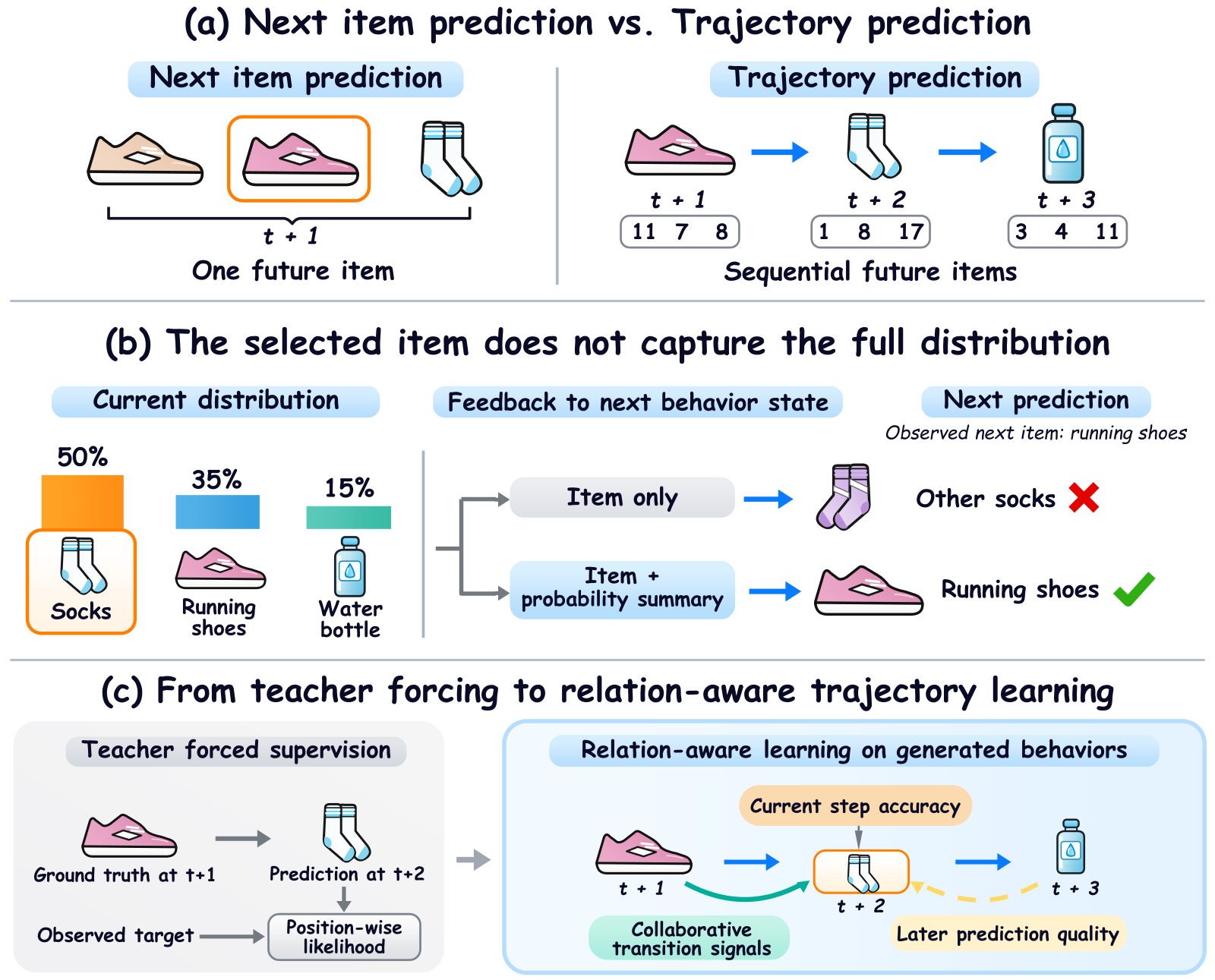
The model was 50% sure about socks. Where did the 35% for running shoes go? How TraGR predicts a user's next several actionsA user has just bought a pair of running shoes. Next they will probably buy sports socks, and then a water bottle. A recommender that only guesses the next item sees just the first step of this path; one that can guess the next few steps in order can prepare related recommendations ahead of time.
Suppose the model is guessing the second step: socks 50%, running shoes 35%, water bottle 15%. It picks socks and moves on to the third step. The trouble is that only "socks" is passed forward. Where did the 35% for running shoes go? With only socks in hand, the model may well guess another pair of socks at step three. Yet this user's actual next action was running shoes.
This paper, from Tongji University, The Chinese University of Hong Kong, Kuaishou Technology and Fudan University, studies user behavior trajectory prediction: given a user's history, predict their next K interactions in order. Most sequential recommenders predict only the next item. Generative recommenders write each item as a short string of discrete codes, a Semantic ID (SID), and generate the codes one by one. GCB, an SID-based trajectory generator, extends this to a sequence of items, generating codes item after item; but each item takes several serial decoding steps, only the chosen item is passed on, and training always feeds the true history. TraGR predicts all codes of an item in parallel and updates a "behavior state" once per item. Each update carries the chosen item plus a summary of the candidates weighted by probability and similarity. Finally, it trains on its own generated trajectories so that how well later steps go feeds back into earlier choices. On four public datasets it has the top score in all 36 dataset-metric combinations.
Pass on both "what was chosen" and "what almost was," and let later steps train earlier choices, and the gains are largest at later positions; but the largest catalog in the experiments has only about twelve thousand items, and the candidate summary is computed over the whole catalog at every step.
A sequence of actions is not a candidate list
A next-item list, say running shoes, another pair of running shoes, socks, holds alternatives for a single moment; the user picks one of them. A trajectory holds actions at different moments: step 1 running shoes, step 2 socks, step 3 a water bottle. If an earlier step is wrong, the conditions for the later steps are wrong too.
So evaluation is done per position. At each future position the paper computes HR@10 (whether the true item is in the top 10) and NDCG@10 (higher when ranked higher), then combines positions. Metrics starting with M use the arithmetic mean, such as MNDCG, the arithmetic mean of per-position NDCG; metrics starting with S use the geometric mean, such as SNDCG, the geometric mean of per-position NDCG, and SHR, the geometric mean of per-position HR. The geometric mean is more sensitive to one especially bad step. SeqMatch@50 is stricter: a trajectory counts only if the true item at every position is in that position's top 50.
Where code-by-code generation gets stuck
In generative recommendation, each item maps to a string of codes; in the figure, running shoes are "11 7 8". The model writes codes one at a time like words in a sentence, completes one item, then moves on to the next.
The paper points to three problems when this is applied to trajectories. First, the same token-by-token process both "spells out this item's codes" and "moves from this item to the next," so each item takes several interdependent decoding steps and the transitions between items are buried in a long string of codes. Second, the chosen item has not actually been observed yet; passing only that item forward throws away the model's judgment about the other candidates. Third, during training the next step is always conditioned on the true history, while at inference it is conditioned on the model's own guesses, so the two do not match.
How TraGR generates one item at a time
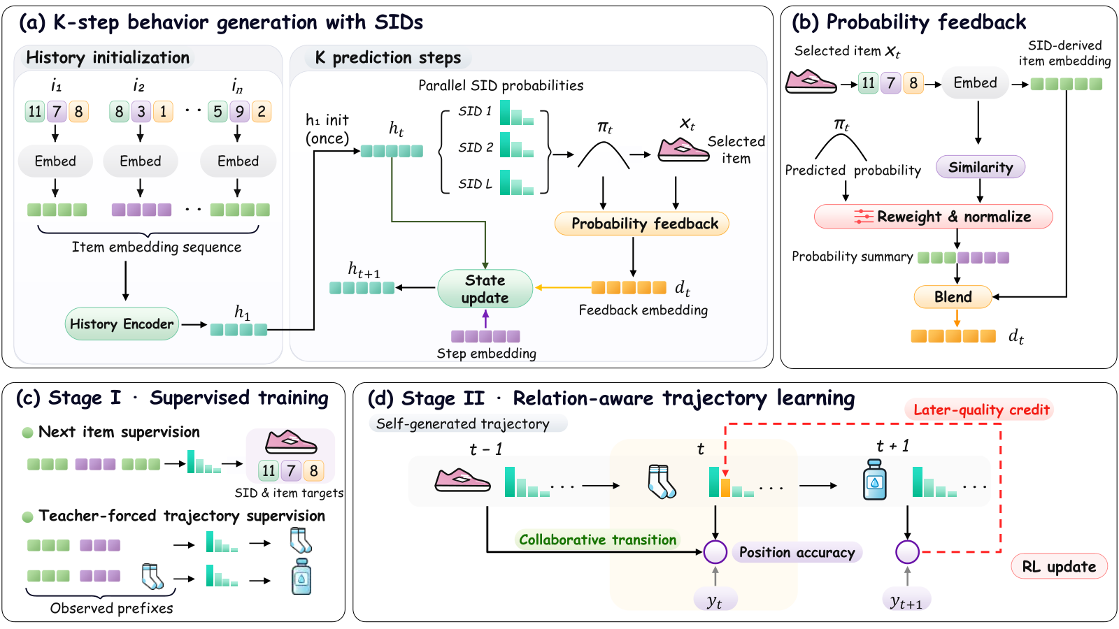
TraGR follows the code scheme of RPG, a generative recommender that predicts codes in parallel: OPQ compresses each item's text features into 16 codes, each position taking one of 256 values. The item vector is the average of its 16 code vectors.
During prediction, the model keeps a behavior state, which can be read as a vector for "where the user is right now." It starts from a Transformer encoding of the history. Each step does the following:
| Step | Input | Output |
|---|---|---|
| Predict codes in parallel | Current behavior state | Code probabilities for each of the 16 positions |
| Build the item distribution | 16 sets of code probabilities | A probability for every item in the catalog |
| Choose an item | Item distribution | At inference, the most likely item |
| Compute feedback | Chosen item + full distribution | A feedback vector |
| Update the state | Old state + feedback vector + step embedding | The next behavior state |
The 16 codes come from 16 small networks at once, not one after another. An item's score is the average log probability of its 16 codes, followed by one softmax over the whole catalog. The state updates once per item, and that update is what carries the transition from one item to the next.
Walking through it: socks 50%, running shoes 35%
Here is how the feedback is computed for the three candidates in the paper's Fig. 1(b). The probabilities 50%, 35% and 15% come from the paper's figure; the similarity factors are illustrative. The mixing coefficient 0.75 is the value the paper uses in stage two and at evaluation.
Step one, choose an item. The distribution at step two is socks 0.5, running shoes 0.35, water bottle 0.15. At inference the most likely item is chosen: socks.
Step two, reweight the candidates. Each candidate's weight is "its probability × its similarity factor to socks," then normalized. Illustration: similarity factors socks 1.0, running shoes 0.5, water bottle 0.2. The products are 0.5, 0.175 and 0.03, summing to 0.705; normalized, that is socks 0.71, running shoes 0.25, water bottle 0.04. The water bottle, unrelated to the chosen item and unlikely, gets pushed down.
Step three, blend into the feedback vector. Feedback vector = 0.25 × socks vector + 0.75 × candidate summary. Plugging in, socks make up 0.25 + 0.75 × 0.71 ≈ 0.78 of the feedback, running shoes 0.75 × 0.25 ≈ 0.19, and the remaining 0.03 or so is the water bottle. This means running shoes still keep nearly a fifth of the feedback; passing only the chosen item would give socks everything and running shoes nothing.
Step four, the feedback updates the state. The next behavior state = current state + a small network's output on "current state, feedback vector, step number." The 0.19 of running shoes enters the state, so at step three the model still remembers that "running shoes were quite likely too."
Step five, gradients flow back along the same path. The summary weights contain the step-two probabilities, so the step-three loss can travel back through the feedback vector and adjust the probabilities step two gave to running shoes and socks. The paper cut this path as a control: SNDCG@10 on Beauty fell from 0.0296 to 0.0281.
The example shows that the feedback vector is a mix of the chosen item and its "runners-up": similarity decides which runners-up stay, probability decides how much. The paper's ablation separates these pieces. On Beauty, passing only the chosen item gives SNDCG@10 of 0.0273; adding a summary weighted by probability alone raises it to 0.0281; weighting by similarity alone drops it to 0.0262; using probability and similarity together raises it to 0.0296. Removing the 0.25 share of the chosen item itself from the feedback drops it to 0.0292.
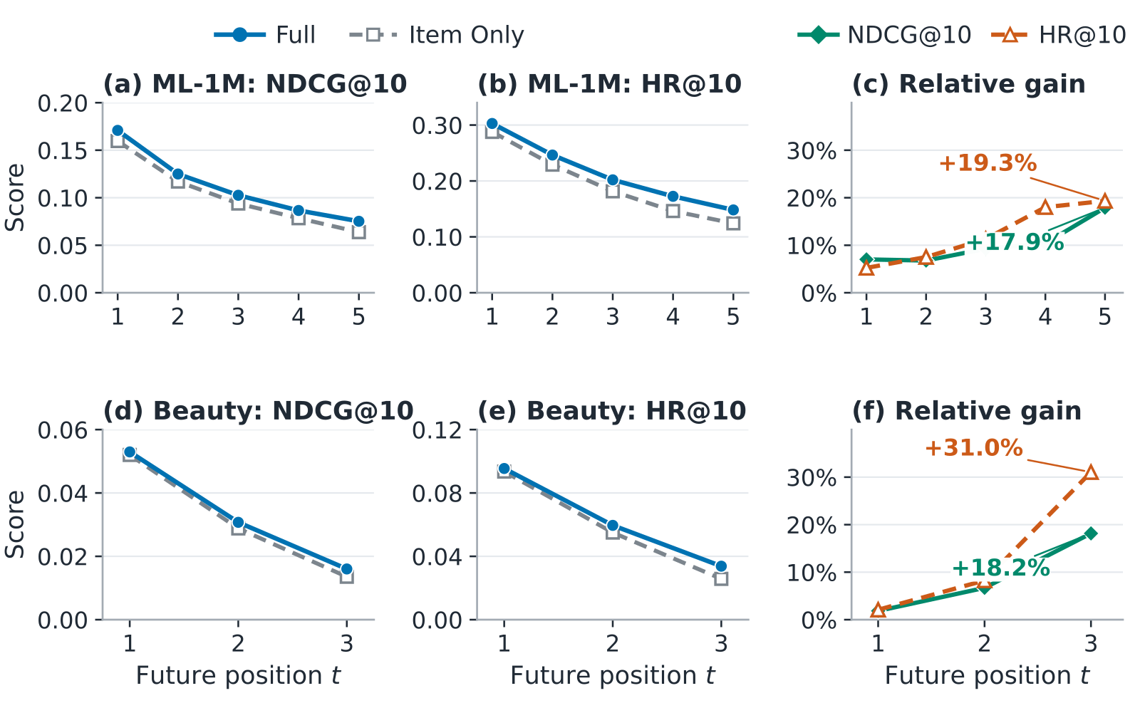
The benefit shows up mostly at later steps. On ML-1M, the relative HR@10 gain grows from about 5% at step 1 to 19.3% at step 5; on Beauty, the relative HR@10 gain at step 3 is 31.0%. This shows probability feedback mainly helps the later steps of a trajectory, which is also how the paper reads it.
Training again on its own trajectories
Stage one is ordinary supervised training: predict the next item, and also train on the true following items with the true history fed in. Here the feedback uses only the chosen item; the mixing coefficient is 0.
Stage two turns on probability feedback and switches to trajectories the model generates itself. For each history, the model samples 8 trajectories from its own distribution, and the true future actions are used only for scoring. At each step, every candidate's reward has two parts: 1 for hitting the true item at that position, plus 0.25 times a "collaborative transition score," which is the fraction of users in the training data who, starting from the previous item, went next to exactly this item. The sum is divided by K.
This reward can be computed for every item in the catalog, so the model directly optimizes the expected reward at each step, and items that were not sampled still receive gradients. In addition, the item chosen at one step changes the conditions for the later steps. The paper sums the expected rewards of the later steps, subtracts the average total reward of the other trajectories for the same history, and uses that as extra credit for this step's choice: if the rest of the trajectory went better than the others, this step's choice is reinforced. A KL term keeps the model from drifting too far from the stage-one model.
The paper compares removing each of these in Table V: taking either the collaborative transition score or the later-step credit out of the full version lowers every metric. Just doing more supervised training, or continuing supervised training on sampled prefixes, does not match the full version.
Results
The paper uses four public datasets: Beauty, Cell Phones, ML-1M and Last-FM. The first two have short user sequences and predict 3 steps; the last two have long sequences and predict 5. There are 13 baseline configurations, covering classic sequential recommenders, diffusion models, generative recommenders, and the dedicated trajectory methods LPDO (which generates trajectories with a diffusion model) and GCB. GCB has no public code; the authors reimplemented it from its paper.
| Dataset | Items | Strongest baseline (SNDCG@10) | TraGR | Relative gain |
|---|---|---|---|---|
| Beauty | 12,101 | RPG-M 0.0251 | 0.0296 | 17.9% |
| Cell Phones | 10,429 | EchoRec 0.0193 | 0.0229 | 18.65% |
| ML-1M | 3,706 | LPDO 0.0936 | 0.1074 | 14.7% |
| Last-FM | 987 | TIGER 0.2019 | 0.2052 | 1.63% |
(Numbers from the paper's Tables I and III; relative gains computed from the table values.)
This shows TraGR beats the strongest competitor on each of the four datasets, and that competitor is different on each one. SeqMatch@50 also improves on all four datasets, by about 29.46%, 75.65%, 6.63% and 12.02%, and on three of them the relative gain exceeds that of SNDCG@10: more users have every step of their trajectory in the top 50. Absolute values are still low: SNDCG@10 on Beauty is under 0.03.
When the horizon is stretched to 7 and 10 steps, every method gets worse; compared with LPDO and GCB, TraGR drops the least from 3 to 10 steps. The one exception is Last-FM at 3 steps, where LPDO's SNDCG@10 is slightly higher. In inference time, TraGR is faster than LPDO and than GCB with its step-by-step decoding, but slower than RPG; it uses less GPU memory than GCB but more than LPDO and RPG.
What this means for people building generative recommenders
If your generative model rolls forward step by step, do not pass on only the argmax item.
One change you can borrow is the paper's "probability summary": mix a share of the runner-up items, weighted by probability and similarity, into the vector passed to the next step. In the ablation, adding a summary weighted by probability alone improves every metric on both Beauty and ML-1M; adding similarity and the chosen item itself improves it further.
The training recipe is also worth borrowing. Training only on true histories means the model never sees what happens after its own wrong guesses; training on its own sampled trajectories, and crediting earlier choices with how the later steps went, is one concrete way the paper offers.
Limitations
The largest catalog in the experiments has 12,101 items. The candidate summary takes a weighted sum over the whole catalog at every step, so its cost grows in proportion to the number of items. The paper itself lists reducing this cost for larger catalogs as future work.
All results are offline metrics, with no online experiment. GCB, the most relevant trajectory baseline, has no public code and was reimplemented by the authors.
A larger mixing coefficient is not always better: on ML-1M, raising it from 0.75 to 0.90 keeps raising SNDCG@10 but lowers SHR@10. Adding the collaborative transition score alone, or the later-step credit alone, gives mixed results across datasets; only the two together are consistently better.
How did this read for you?
Hoot made a note. Thanks for the feedback.

One tap, no sign-in; tap again to undo. Only anonymous counts are kept, never who you are.
Related papersMore from Paper Daily
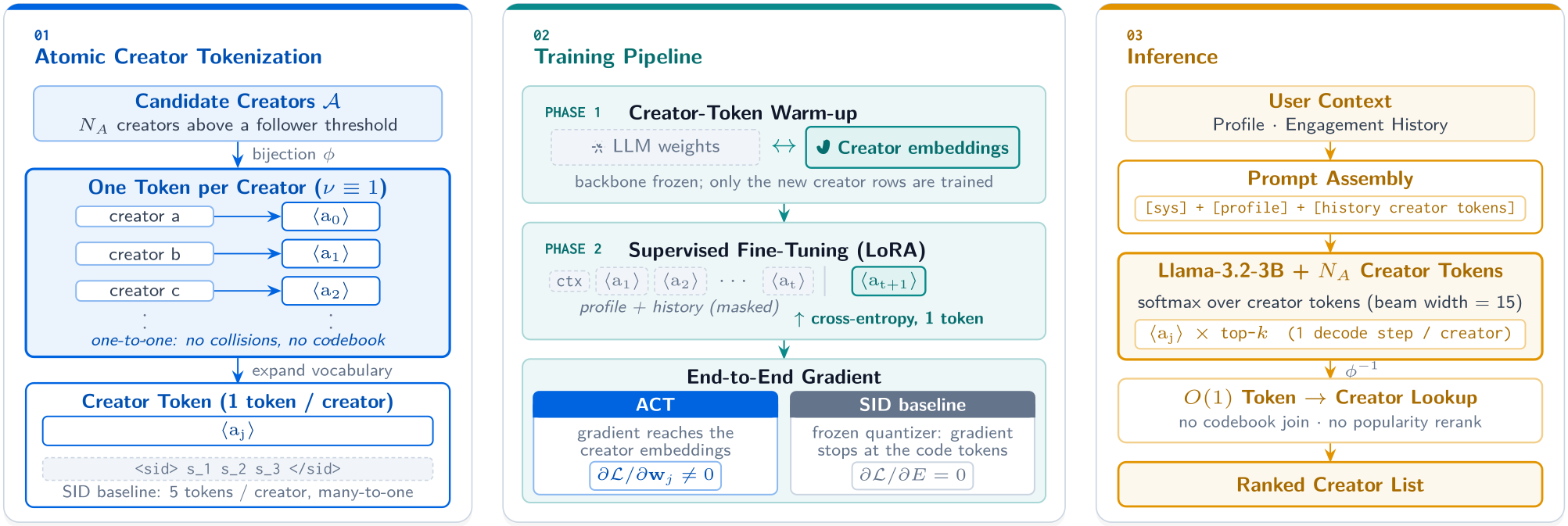 Generative · 2026-11-04Beyond Semantic IDs: Atomic Creator Tokens for Large-Scale Generative RecommendationThis Meta paper gives every creator its own token in the language model's vocabulary and uses it in place of the SID. The reason is simple: an SID is a many-to-one code, so several creators share one SID, and even when the model generates the right SID it still has to guess which of those creators the user wants. On Meta's creator recommendation data, swapping only the token layer lifts the share…
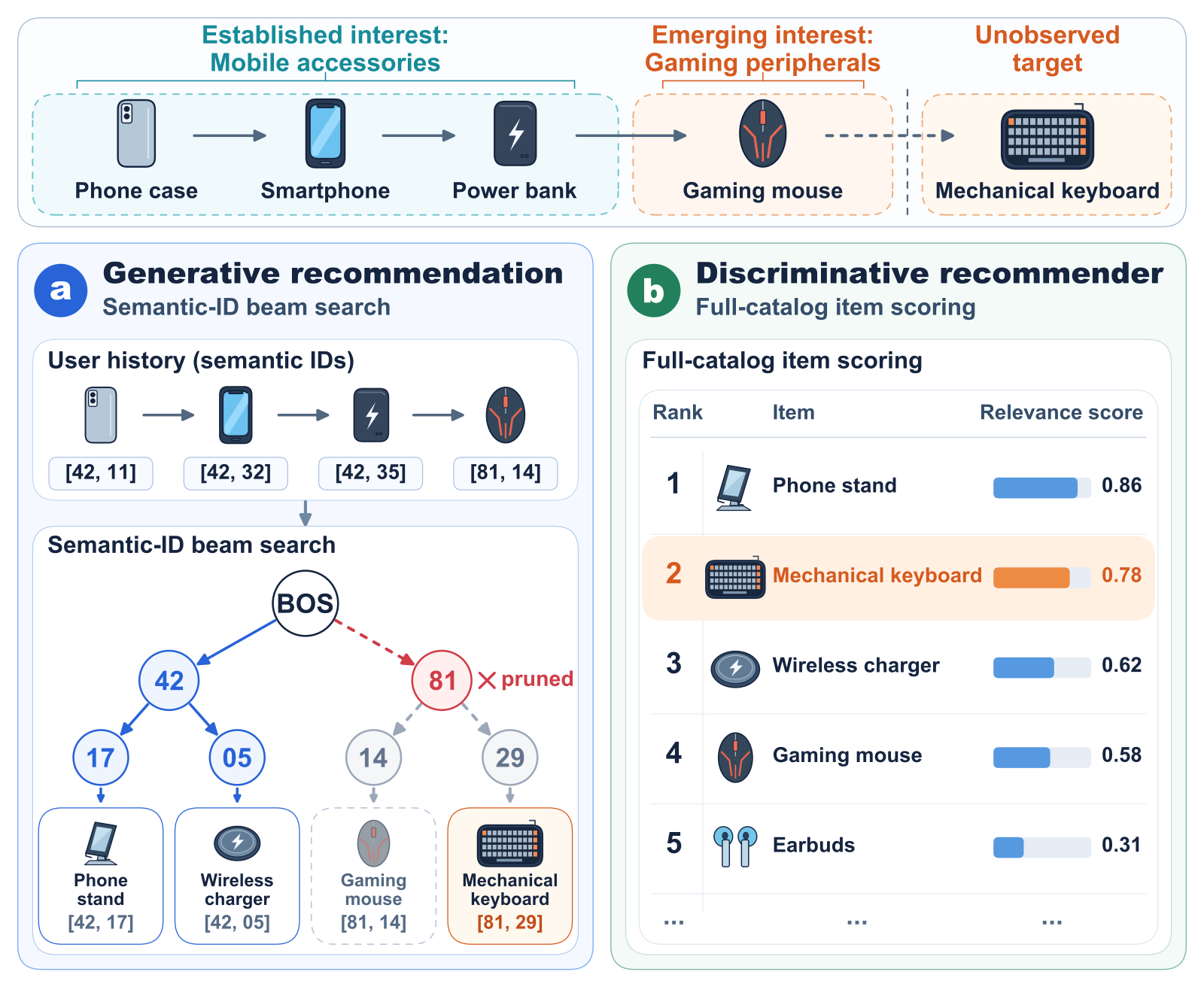 Generative · 2026-10-26From Item Scores to Semantic Tokens: Test-Time Collaborative Adaptation for Generative RecommendationIn generative recommendation with semantic IDs, the model writes an item's code one token at a time, and beam search keeps only the highest-scoring prefixes at each step. Once a prefix is pruned, every item beneath it can never be generated. The problem is sharpest when a user has just developed a new interest that shows up in only one or two recent interactions. This paper proposes TCBSA (test-t…
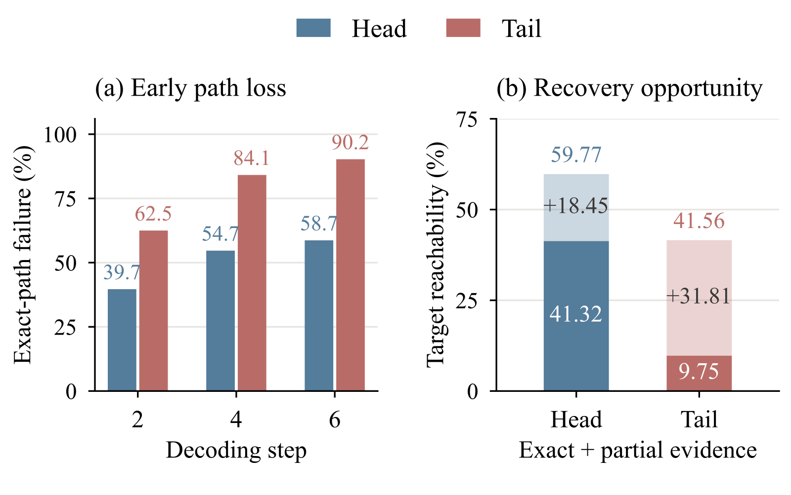 Generative · 2026-11-16ReSID: Rethinking Long-Tail Retrieval in Generative Recommendation through Item ReachabilityGenerative recommendation encodes each item as a string of Semantic ID tokens and generates them one position at a time with beam search, and cold long-tail items are hard to retrieve this way. The authors take apart the whole chain from encoding through decoding to matching and find that tail items are mostly lost early in decoding: on Amazon Industrial, 62.5% of tail targets have already fallen…
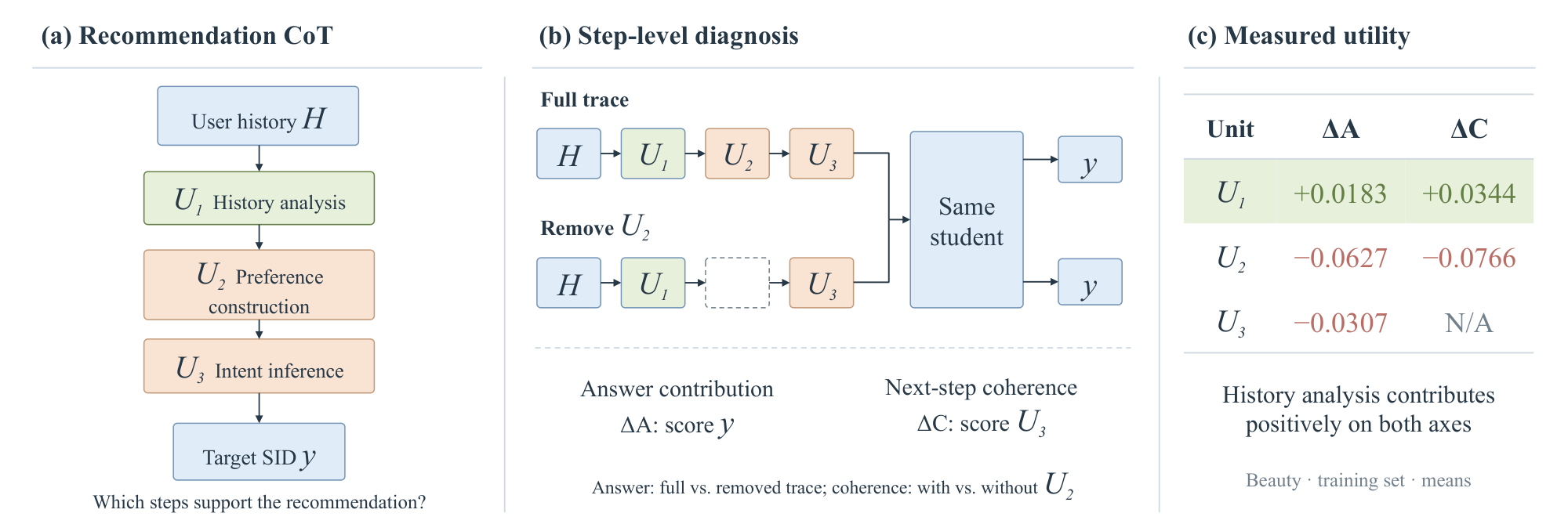 Generative · 2026-11-10Rethinking Latent Reasoning for Generative Recommendation: Beyond Teacher-Generated CoT and Recurrent Hidden-State FeedbackLatent reasoning for generative recommendation usually needs a teacher model to write chain-of-thought traces, which is costly and hard to stabilize. This paper skips teacher generation. It builds semantic targets from the text meaning of items already in a user's history, and uses those targets to supervise the model's intermediate tokens that are reserved for reasoning steps, without looking at…
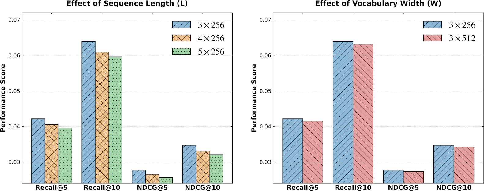 Generative · 2026-08-21Semantic Trimming and Auxiliary Multi-step Prediction for Generative RecommendationDeep dive: Semantic Trimming and Auxiliary Multi-step Prediction for Generative Recommendation.
 Generative · 2026-11-06BRIDGE: Bridging the Semantic Quantization Gap for Generative RecommendationGenerative retrieval predicts the next item's Semantic ID (SID) one code at a time from user history, but ordinary next-code training checks only the probability assigned to the correct code. When that probability stays the same, redistributing the remaining probability among incorrect candidates does not change this cross-entropy loss. BRIDGE (the generative retrieval model studied here) also us…
 Generative · 2026-11-02Towards Reliable, Scalable, and Value-Aligned Generative Recommendation for Large-Scale AdvertisingKuaishou made three changes to GR4AD, its deployed generative ad retrieval system, and the result, GR4AD-X, raises online ad revenue by a cumulative 3.07% over GR4AD. All three target the same mismatch: the model picks ads by generation probability, while the platform cares about revenue. The top ten ads by generation probability and the top ten by eCPM barely overlap, with a hit rate of only abo…
 Generative · 2026-10-21AGR: Agentic Generative Retrieval with Tool-Augmented SearchGenerative retrieval need not encode every available feature up front. AGR requests intent, location, or behavioral evidence while decoding item identifiers, then resumes generation with a compact observation. A Kuaishou online experiment reports a 0.205% increase in requests with strongly relevant top-four results.
Discussion
Add experiment details, reproduction notes or a different take. Requires a GitHub sign-in.
Loading the discussion…