Contents · 10 sections
1What problem is it actually solving?2The whole picture first3Input side: which tokens to drop4Output side: predict one more token5Results: how much faster, and was accuracy lost?6What each part does7How much to prune, and at which layer8Where I think it falls short9How a generative-recommendation team could try it10Verdict and scorecardSHARE

Teams that run Semantic-ID generative recommendation and are limited by training cost should read this, but with some questions in mind. It deals with a practical tension: once every item is split into three or more SID tokens, user histories grow several-fold, training gets slow and memory-hungry, and many of the extra tokens are repeated category and brand codes. The core idea of STAMP (the authors' training framework): at some middle layer of the Transformer, score every token by "its own activation strength × how much attention other tokens pay to it", and pass only the high scorers on to later layers. A training-only loss that predicts one token further ahead then wins back what pruning lost. On three Amazon datasets it raises training speed by 1.36–1.38× and cuts peak GPU memory by more than 52%, with Recall@10 on par with the original model. On AL-GR-Tiny, industrial data released from a large Chinese e-commerce platform, it is 1.34× faster but saves only 17.2% of memory.
What problem is it actually solving?
Generative recommendation treats "recommend the next item" as generation: the model reads the user's history and emits the target item's identifier token by token. Early systems gave each item its own ID, which meant huge vocabularies and no way for a new item to share information with old ones. The mainstream now is Semantic IDs (SIDs): embed each item with a text model, then quantize the embedding layer by layer with RQ-VAE or RQ-Kmeans into a few discrete codes. The first code roughly corresponds to a category, and later codes get finer. Similar items share prefixes, which helps cold start and generalization.
The price is longer sequences. An illustrative example:
| Items the user bought recently (illustrative) | As a single ID | As 3 SID tokens |
|---|---|---|
| Brand-A moisturizing cream | 1 token | skincare · brand A · cream |
| Brand-A toner | 1 token | skincare · brand A · toner |
| Brand-A serum | 1 token | skincare · brand A · serum |
| A lipstick | 1 token | makeup · brand B · lipstick |
Four items go from 4 tokens to 12. In the paper's GRID setup (GRID is an open-source SID generative-recommendation framework) the input is 120 tokens with 3 codes per item, which by my arithmetic is the last 40 items. Attention cost grows with the square of length, so memory and training time grow with it. Note also that "skincare" and "brand A" each appear three times. The first occurrence tells the model this user likes skincare and brand A; the next two add much less.
The authors also see a second problem: finer SIDs can make results worse.
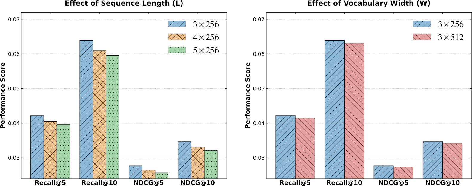
In the left panel Recall@10 falls from about 0.064 with 3 levels to about 0.060 with 5 (read from the chart). The authors trace both problems to one cause they call "semantic dilution": the finer the split, the more low-value, repeated tokens in the input, while the supervision still comes only from the single target item at the end and does not grow with the sequence. The first wastes compute; the second makes it harder to find the few tokens that actually drive a purchase in a long history.
The whole picture first
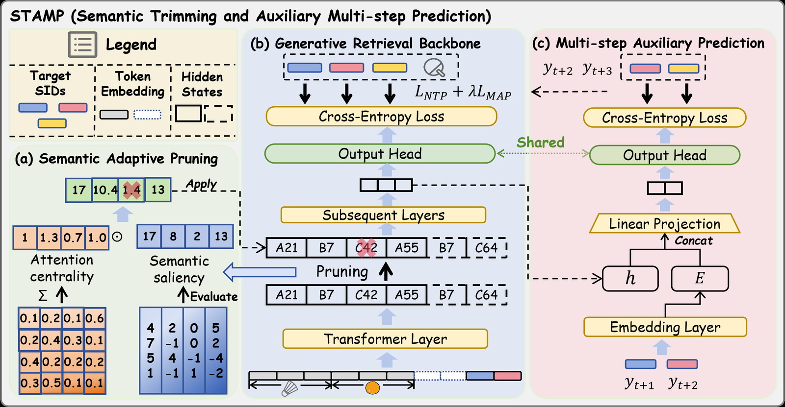
STAMP has two independent parts: a pruning part, SAP (Semantic Adaptive Pruning), and an auxiliary-prediction part, MAP (Multi-step Auxiliary Prediction, unrelated to the retrieval metric MAP). Training works like this:
| Step | What happens | Output |
|---|---|---|
| 1. First layers | Process the full SID sequence as usual | Hidden states and attention weights for every token |
| 2. Pruning layer (SAP) | Score each token, keep the top fraction α, restore the original order | A shorter sequence |
| 3. Remaining layers | Process only the kept tokens | Hidden states that predict the target item's SID |
| 4. Loss | Usual per-token cross-entropy plus λ times the auxiliary loss (MAP) | Gradients |
The key division of labor: pruning only saves compute, and auxiliary prediction only densifies supervision. Now the parts one by one.
Input side: which tokens to drop
Why prune inside the model instead of just truncating the input? Because in a SID sequence you cannot tell in advance which token is useless. Natural language has filler words you can delete; every SID token is a meaningful code. So the model runs a few layers first and then decides what to drop using signals it has computed itself.
Each token's score is a product of two parts. The first is semantic saliency: the sum of absolute values (ℓ1 norm) of the token's hidden vector at the pruning layer, normalized; larger means stronger activation. The second is attention centrality: the attention weight the token receives from all other tokens across all heads, summed; larger means other tokens draw on it more often.
Here is token i's final score, the semantic saliency and the attention centrality. The intuition behind multiplying: a token is worth keeping only if it carries a lot of information itself and is also frequently referenced by others.
The left of the framework figure is a worked example you can do by hand. Four tokens have centrality 1, 1.3, 0.7, 1.0 and saliency 17, 8, 2, 13; the products are 17, 10.4, 1.4 and 13. The third token is low on both and scores only 1.4, so it is pruned. By centrality alone the second token (1.3) would rank first; after multiplying by saliency it ranks third.
Two details follow the selection. First, the kept tokens are re-sorted by original position before their hidden states are gathered, so the order of the history is preserved. Second, kept tokens keep their original position ids instead of being renumbered from zero. Models with RoPE, such as Qwen, therefore still know how far apart two now-adjacent tokens originally were. In a decoder-only model like Qwen the target item sits in the same sequence as the history, so the authors always keep the target item's tokens, outside the scoring. Otherwise a target token could be pruned and its gradient would have nowhere to go.
This step adds no parameters; the scores reuse attention weights the backbone has already computed. The keep ratio is α=1/3 on T5, so two thirds are pruned, and α=0.6 on Qwen.
Output side: predict one more token
Pruning loses information, which makes it harder to learn preferences from what is left. The second part adds an auxiliary training objective.
In normal training the target item's SID has 3 tokens and at each step the model predicts only the next one. MAP does one more thing at each step: it takes the hidden state at the current position, , concatenates the embedding of the next true token , passes it through an MLP, and uses the backbone's output head to predict the token after that, .
is the usual per-token cross-entropy, the cross-entropy of predicting one step further, and λ is 0.3.
Walk through it with the illustrative item above, where the target is "makeup · brand B · lipstick". Normal training has 3 predictions: "makeup" from the history, "brand B" from the history plus "makeup", then "lipstick". MAP adds 2 more. At the position that predicts "makeup", it feeds in the true "makeup" and asks for "brand B". At the position that predicts "brand B", it feeds in the true "brand B" and asks for "lipstick". The hidden state responsible for the first code now also has to carry information useful for the later codes.
Why feed the true token rather than the model's own prediction? Because the prediction may be wrong, and a wrong input would teach the auxiliary objective noise. This matches how DeepSeek-V3's MTP module works. The auxiliary module is a single MLP, the output head is shared with the backbone, and the whole thing is removed at inference, so it adds no serving latency.
Results: how much faster, and was accuracy lost?
The authors ran experiments on two architectures. One line uses a small T5 on GRID: 4 encoder and 4 decoder layers, hidden size 128, on Amazon Beauty, Sports and Toys, with the last interaction held out for testing and results averaged over 5 random seeds. The other uses Qwen2.5-0.5B on FORGE (a SID generative-recommendation benchmark framework aimed at industrial settings) with AL-GR-Tiny: data from a large Chinese e-commerce platform, four days of behavior for training and the fifth day for testing, run once. The only comparison method is EARN (an inference-acceleration method): it places one learnable "register" token before and one after the history; in the first layers these two read the whole history through attention, and at a chosen layer all history tokens are dropped so later layers see only the two registers. EARN was built for faster inference and is used here to speed up training. L=1 means pruning or compression after layer 1.
| Dataset | Metric | Original | EARN | STAMP | STAMP speedup / memory cut | EARN speedup |
|---|---|---|---|---|---|---|
| Beauty (T5, L=1) | Recall@10 | 0.0645 | 0.0591 | 0.0657 | 1.38× / 53.3% | 2.16× |
| Sports (T5, L=1) | Recall@10 | 0.0354 | 0.0311 | 0.0354 | 1.36× / 54.7% | 2.16× |
| Toys (T5, L=1) | Recall@10 | 0.0499 | 0.0415 | 0.0509 | 1.36× / 52.1% | 2.20× |
| AL-GR-Tiny (Qwen, L=6) | Hit@1000 | 0.1400 | 0.1021 | 0.1405 | 1.34× / 17.2% | 2.62× |
| AL-GR-Tiny (Qwen, L=6) | Hit@20 | 0.0209 | 0.0152 | 0.0207 | same | same |
The table shows two things. First, EARN is much faster, but squeezing the whole history into two tokens costs too much: Recall@10 drops 17% on Toys and Hit@1000 drops 27% on the industrial data. STAMP keeps original tokens, only fewer of them, so accuracy mostly holds. Second, the gap between STAMP and the original model is within random variation. On Beauty, STAMP's Recall@10 is 0.0012 higher, while the two standard deviations are 0.0022 and 0.0019, so this counts as a tie, not an improvement.
Why only a bit over 1.3× when two thirds of the tokens are pruned, rather than 3×? Layer 1 still processes every token, and the decoder is untouched; pruning only saves the later encoder layers. On Qwen memory drops only 17.2%, for two reasons. α=0.6 is conservative, and the 0.5B model has 24 layers whose parameters and optimizer state take fixed memory; pruning tokens only reduces the activations that scale with sequence length.
What each part does
The authors measured the efficiency of the two parts separately:
| Setting (Beauty, T5) | Training time | Speedup | Peak memory cut |
|---|---|---|---|
| Original | 212s | – | – |
| MAP only | 216s | 0.98× | about 0% |
| SAP only (L=1) | 146s | 1.45× | 53.3% |
| STAMP (L=1) | 154s | 1.38× | 53.3% |
All of the speedup comes from pruning; auxiliary prediction makes training about 2% slower. On Qwen the auxiliary MLP's input is twice the 896 hidden size, and memory actually rises by 2.42%.
On accuracy, the authors find on the three Amazon sets that MAP alone beats the original model, SAP alone is usually slightly worse (Beauty and Toys get slightly better when pruning at layer 2), and the two together sit in between, close to the original. The ablation on the industrial data deserves its own look:
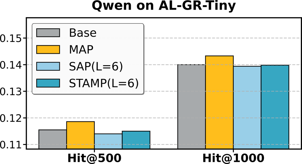
Reading the chart, MAP alone reaches about 0.143 Hit@1000, the original 0.140, and STAMP about 0.140. So on the industrial data, the gain from MAP is cancelled out by pruning; STAMP is essentially "trading MAP's gain for 1.34× faster training". The STAMP bar for Hit@1000 also looks slightly below 0.14, which does not quite match the table's 0.1405; keep that discrepancy in mind when quoting either number.
How much to prune, and at which layer
On Qwen the authors swept the pruning layer (1, 2 or 6) and the keep ratio α (0.33 to 0.95):
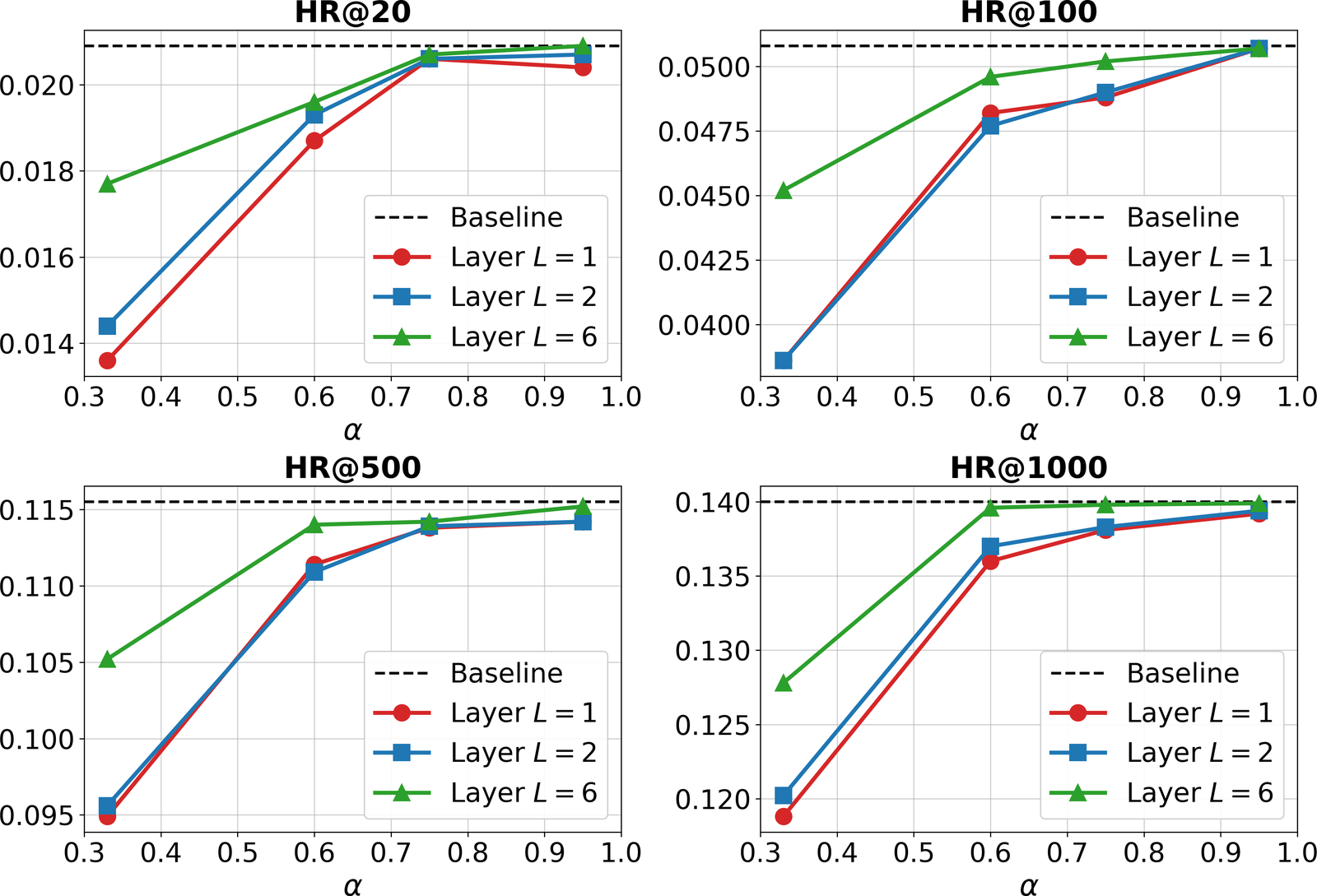
The figure says two things. First, when 60% or more of the tokens are kept, the pruning layer barely matters and results stay close to the original, so a real share of tokens can indeed go. Second, under aggressive pruning, later is better: at α=0.33, HR@20 when pruning at layer 6 is about 30% higher than at layer 1 (read from the chart).
The authors explain this with attention heatmaps. Some tokens get heavy attention in shallow layers and almost none in deep layers. They work like scaffolding: shallow layers use them to gather information into a few key tokens, and once that is done they can be removed. Pruning too early throws their information away before it has been absorbed. The T5 experiments also compare scoring rules: scoring by the hidden vector's ℓ2 norm alone, or by attention centrality alone, both lose to the product, with the gap widening late in training. The first drops positions whose own values are small but which many tokens attend to; the second misses positions that gather information gradually in deeper layers.
Where I think it falls short
First, the speedup figure is optimistic. Speed is measured as the time for a fixed 1,600 steps, but the GRID runs use early stopping and the authors themselves say the total step count varies with method and seed. If the pruned model needs more steps to converge, 1.38× faster per step is not 1.38× faster training. The paper gives per-step time; total time to convergence has to be measured on your own data.
Second, the simplest controls are missing. The only baseline, EARN, is an inference method that compresses very aggressively. The comparison that matters is the naive one with the same budget: keep only the most recent 40 tokens, or randomly drop two thirds. Without those, we cannot tell how much better "own activation × attention received" is than simply cutting old history. The pruning-strategy comparison also covers only pooling and single signals, not recency truncation.
Third, the evidence on industrial data is the weakest. AL-GR-Tiny was run once, STAMP and the original differ by at most 0.0006 on all four Hit metrics, so significance cannot be judged, and MAP alone is actually the best variant. Memory savings also shrink from over 50% on T5 to 17.2%, and will shrink further for bigger models. All speed and memory numbers in the paper are for training; savings at inference also have to be measured yourself.
How a generative-recommendation team could try it
- Diagnose before changing training. In an existing SID model, sum the attention each token receives at a middle layer and sort from high to low. Compute what share of all attention goes to the bottom two thirds of tokens, and check whether they cluster on repeated category and brand codes. If the bottom two thirds still receive a sizable share, most tokens are in use, there is little room for pruning, and you can stop here.
- Add MAP alone. It is one MLP; start with λ=0.3, at roughly 1–2% more training time. On the industrial data this was the most accurate setting, so check whether offline Recall or Hit improves consistently.
- Then add pruning, together with a control that keeps only the most recent α·N tokens at the same ratio. Start at α=0.6, pruning at about a quarter of the depth, and compare total GPU time to convergence, not per-step time.
- For decoder-only models with RoPE, keep the original position ids and always keep the target segment; otherwise position relations and gradients break after pruning.
Verdict and scorecard
The key lesson: repeated category and brand codes in SID sequences can mostly be dropped safely in the middle of the model, but only after the shallow layers have gathered their information.
| Dimension | Assessment |
|---|---|
| Importance of the problem | High. SIDs make sequences several times longer, and training cost is a real bottleneck for deploying generative recommendation |
| Novelty of the method | Medium. Both the scoring and the multi-step prediction come from existing LLM acceleration work; the contribution is combining them for SID training and handling order and positions correctly |
| Strength of evidence | Medium-low. One inference-oriented baseline, no recency-truncation control, and the industrial data was run once with tiny gaps |
| Engineering cost | Low. Pruning adds no parameters, the auxiliary module is one MLP and can be removed at inference |
| Worth trying? | Yes, cheaply. Try MAP alone first, then pruning with a truncation control |
| Where it fits | Generative retrieval that represents long user histories with multi-level SIDs and retrains often |
How did this read for you?
Hoot made a note. Thanks for the feedback.

One tap, no sign-in; tap again to undo. Only anonymous counts are kept, never who you are.
Related papersMore from Paper Daily
 Generative · 2026-11-04Where Beam Search Loses Top-Ranked Items:First-Step Coverage in Generative RecommendationA generative recommender uses beam search to produce a SID one token at a time, and the usual way to miss fewer good results is to widen every step at once. This paper checks six full-test settings of TIGER one by one: every result that the model's own scores put in the top 10, but that beam search pruned, was lost at the very first step. So the cheaper move is to concentrate width on the first s…
 Generative · 2026-11-16From Tokens to Behaviors: Rethinking Generative Recommendation for User Trajectory PredictionMost recommenders guess only the user's next click, while user trajectory prediction guesses the next several steps at once, such as buying running shoes and then sports socks and a water bottle. Generative recommendation does this by generating each item's SID token by token before moving to the next item, so the encoding within an item and the transitions between items are tangled in one chain.…
 Generative · 2026-11-11Not All Branches Are Equal: Adaptive Semantic ID Construction for Generative RecommendationGenerative recommendation numbers products with SIDs, and the dominant approach is residual quantization: each level has one global code table and looks up whatever the previous level left unexplained, which amounts to assuming that each token carries its own independent meaning. The authors checked RQ-VAE IDs on Amazon Beauty. Two products sharing only the first token have a mean cosine similari…
 Generative · 2026-11-06BRIDGE: Bridging the Semantic Quantization Gap for Generative RecommendationGenerative retrieval predicts the next item's Semantic ID (SID) one code at a time from user history, but ordinary next-code training checks only the probability assigned to the correct code. When that probability stays the same, redistributing the remaining probability among incorrect candidates does not change this cross-entropy loss. BRIDGE (the generative retrieval model studied here) also us…
 Generative · 2026-11-04Beyond Semantic IDs: Atomic Creator Tokens for Large-Scale Generative RecommendationThis Meta paper gives every creator its own token in the language model's vocabulary and uses it in place of the SID. The reason is simple: an SID is a many-to-one code, so several creators share one SID, and even when the model generates the right SID it still has to guess which of those creators the user wants. On Meta's creator recommendation data, swapping only the token layer lifts the share…
 Generative · 2026-11-04Utility-Aware Generative Recommendation: Utility-Enriched Semantic Codes and Utility-Guided DecodingThis Kuaishou paper adds video utility to two places in generative recommendation that used to look only at content and probability. 3 bits inside the last SID token record the video's utility tier: 7 ascending boundaries cut one utility statistic (such as historical click rate) into 8 tiers. At every beam-search step a small module reads the decoder hidden state, predicts behaviors such as watch…
 Generative · 2026-10-29REGER: Modeling inter-item Relations with Semantic IDs for Generative RecommendationCross-entropy tells a generative recommender only which token is correct, with no signal about how other candidates compare. REGER, from the University of Electronic Science and Technology of China, splits a conventional sequential model's scores over all items into branch preferences along the SID prefix tree and distills them along the true path. Added alone to TIGER, it lifts Beauty Recall@10…
 Generative · 2026-10-28MuSID-KD: Multigranularity Knowledge Distillation for Generative Recommendation with Semantic IDsWhen a SID-based generative recommender is distilled into a small model, the student is usually asked only to match the teacher's distribution over which item to recommend in the end. ECNU's MuSID-KD (a multi-granularity distillation method that works level by level over the SID) finds this is not enough: a student aligned only on items disagrees with the teacher on the order of candidate groups…
Discussion
Add experiment details, reproduction notes or a different take. Requires a GitHub sign-in.
Loading the discussion…