Contents · 7 sections
1When A searches "beef" once, what steps does the request go through from arrival to candidates?2After writing location into the merchant ID, how are beam slots saved?3For the same "beef" search, how does the model rank fresh groceries above hot food?4When the beam fills up with stores of the same chain, whom should we reward?5Why does TS-GEAR lead by more than 30% at 20 km but barely at 5 km?6Removing which component makes HR@50 drop the most?7How much did it gain online, and who bears the cost?SHARE

The most important change in this Taobao Shangou ad retrieval paper is that the retrieval model, when it generates a merchant ID, first writes "which area the merchant is in" and only then "what the merchant sells", so merchants that cannot deliver rarely get to occupy candidate slots.
Taobao Shangou is an on-demand delivery platform: after a user orders takeout or fresh groceries, a courier usually delivers within an hour. When a user searches here, the ad system first retrieves a batch of merchants and then hands them to the downstream ad ranking and bidding. Unlike ordinary e-commerce, a merchant outside the delivery range is an invalid candidate for this user, and its rank does not matter. The delivery range also changes in real time with courier supply, weather and distance: an address a shop can deliver to right now may be out of reach a little later. So the platform cannot store a fixed "deliverable" flag for each merchant.
Generative retrieval in recent years commonly uses Semantic IDs (SID): each merchant is encoded as a few tokens, for example [17, 203, 88] (illustrative), and merchants with similar content tend to share the leading numbers. The model reads the user history and the query, writes out the SID one token at a time, and beam search keeps the highest-scoring batch of sequences. These tokens come from merchant content or collaborative signals and contain no location. To make sure a merchant can deliver, the system can only wait until the SID is generated, look up the corresponding merchant, and then filter by distance.
The paper uses an example to show what goes wrong. On weekdays user A often orders takeout near the office, and most of A's past orders are hot-food shops such as beef rice bowls. On a weekend morning A opens Taobao Shangou at home and searches "beef", wanting fresh beef to cook. Following the history, the model gives high probability to the rice-bowl shops near the office; these shops are semantically close to "beef" but cannot deliver to A's home.
Illustration: the beam has only 10 slots, shops near the office take 7, and after distance filtering only 3 candidates remain. Those 7 slots are already wasted. The filtering also happens after the model generates and is not part of the training loss, so during training the model is never penalized for occupying those 7 slots.
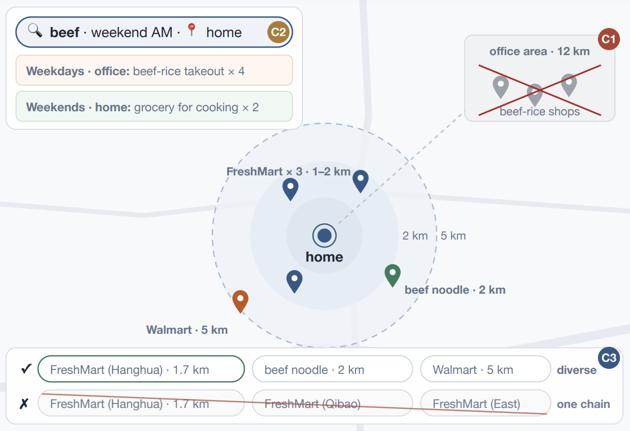
The closest existing approach treats geography as a soft signal, meaning nearby merchants only get somewhat higher scores, with no hard restriction. GNPR (a generative method that builds SIDs for location recommendation) also feeds geographic features as input when compressing merchants into SID codes, and OneLoc biases the model toward nearby merchants during decoding; OneLoc is the strongest scheme of this kind. Back in A's example, a soft signal can push down the probability of the office-area shops somewhat. But A's history contains enough rice-bowl shops that those 7 slots might give up only 2 (illustrative).
The paper's system, TS-GEAR, cuts the map into cells, writes the merchant's cell directly into the merchant ID, and during decoding restricts the start of the ID to the nine cells around the user. Online retrieval only wants merchants within a 20 km radius of the user, and at this radius 95.8% of TS-GEAR's top 50 candidates fall within the radius, versus only 35.4% for OneLoc. Below, "within the radius" and "reachable" are both measured by the distance between merchant and user, while the model constrains the cell the merchant is in. These two ratios describe how many beam slots go to merchants within the radius; how those slots turn into hit rate is worked out later. First, let us follow A's search from start to finish.
When A searches "beef" once, what steps does the request go through from arrival to candidates?
| Step | Input | Operation | Output | When it happens |
|---|---|---|---|---|
| Encode merchant IDs | Merchant latitude and longitude, text description | Convert the location to a geohash cut into three chunks; cluster the content embedding into three codes | A six-token ID, illustrative: [wt, w3, sj, 17, 203, 88] | Offline |
| Aggregate user history | A's real-time location, the query "beef", 100 past behaviors | Compute one similarity by location and one by query for each past behavior, then take a weighted sum | One user representation, read by the decoder (the part of the model that writes the ID token by token) | Training and online |
| Write geographic tokens | A's cell and the 8 surrounding cells | Fill the first two tokens directly with these cells' codes (at most 9 prefixes); the decoder writes the third | The roughly 1.2 km small cell the merchant is in | The first two tokens are filled directly only when decoding candidates; during training the model learns all 6 tokens one by one |
| Write semantic tokens | Geographic prefix, user representation | The decoder goes on to write three semantic tokens | A complete ID; beam search keeps a deduplicated batch of top-scoring IDs as candidates | Training and online |
| Adjust the model by the value of a group of candidates | 8 sampled results for one request, real clicks and orders | GMPO (the paper's reinforcement learning training with a modified reward computation) only rewards samples that hit real behaviors no other sample hit | Updated model | Training only |
| Hand off downstream | Deduplicated candidates | Run in parallel with other retrieval channels such as keyword retrieval and vector retrieval | Enter ad ranking and bidding together | Online |
Training has two stages. The first is pretraining on click logs: the input is a search request, the target is the 6 tokens of the clicked merchant, and the model predicts them one by one. The second is GMPO (the paper's reinforcement learning training with a modified reward computation), which further adjusts the model by the overall value of a group of candidates.
After writing location into the merchant ID, how are beam slots saved?
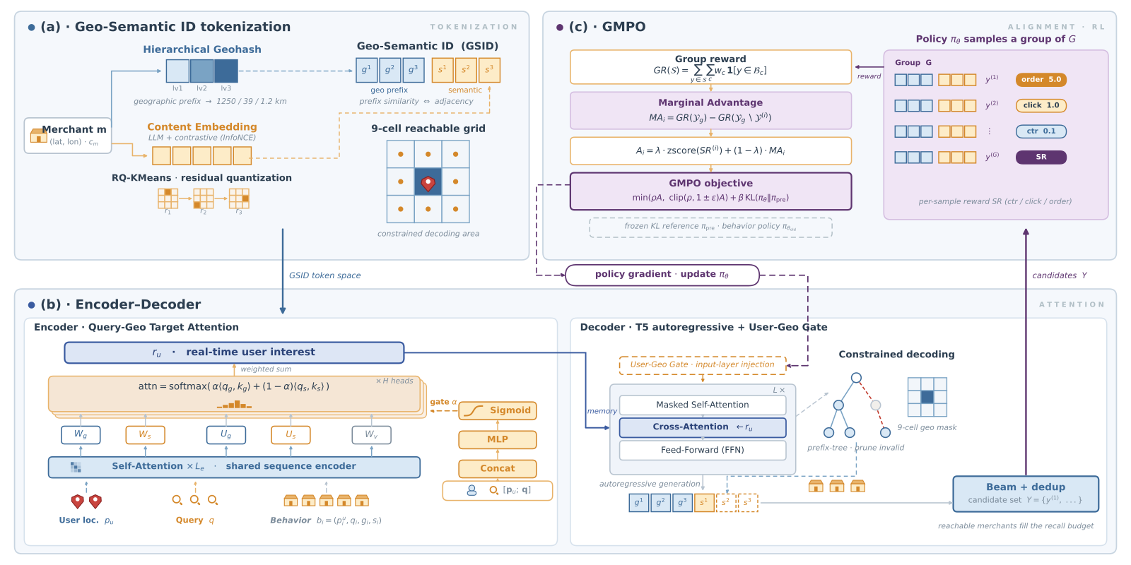
Attaching a "delivery range" attribute to merchants does not work, because the range changes with couriers and weather. Mixing geographic features into SID construction, as GNPR does, is not enough either, because no position in the generated ID stands for geography specifically, so decoding cannot require certain positions to fall near the user. TS-GEAR uses geohash to turn location into a separate segment of the ID.
Geohash cuts the map into nested cells, each cell maps to a string of characters, and cells sharing a prefix are close on the map. The paper uses a 6-character geohash for the merchant location, whose smallest cell is about 1.2 km × 0.6 km. Each geohash character has 32 possible values, and the 6 characters are cut into tokens of two characters each, so each token has 32×32=1024 possible values. The first token alone locates a region of about 1250 km, adding the second narrows it to about 39 km, and all three narrow it to about 1.2 km.
The semantic part follows the usual SID approach. A merchant's region, brand, category and frequent queries are written as a structured text, passed to a fine-tuned Qwen3-Embedding to get an embedding, and then clustered level by level with RQ-KMeans into three codes.
Illustration: fresh-grocery shop B has geohash wtw3sj and content codes 17, 203, 88, so its full ID is [wt, w3, sj, 17, 203, 88]. The paper calls this ID a GSID (Geo-Semantic ID). The first three positions say where the merchant is, and the last three say what it sells.
The decoder writes the ID starting from the first position, so with location at the front of the ID, decoding can restrict the first few positions up front. The first 4 geohash characters of the user's location correspond exactly to the first two tokens of the ID and represent a cell of about 39 km; this cell and its 8 neighbors form a 3×3 grid that essentially covers the platform's maximum delivery radius. Based on A's real-time location, the system looks up these cells' codes, that is, at most 9 prefixes, and treats them as the already-written first two tokens. So of the 6 tokens, the model only has to write 4 itself.
Illustration: without restriction, the first two tokens have 1024×1024, about 1 million combinations, and beam slots may be spent on prefixes of merchants in other cities. With the 3×3 grid, this step has at most 9 combinations, and merchants in other cities cannot enter the beam.
The 3×3 grid does not block every shop outside the radius. Nine cells of about 39 km together are much larger than a 20 km radius. If the office is 30 km from A's home (illustrative), the rice-bowl shops near the office are likely still inside the grid. The office and the home fall in different cells of about 1.2 km, so whether these shops are avoided depends on the third geographic token, that is, the small cell the decoder has to write.
During training the target sequence is a merchant the user actually clicked, so the third token learns which small cell the merchants clicked by users standing at this location usually fall in. User-Geo Gate (a gate in the decoder that adjusts the input by the user's location) adds the user's real-time location to the steps that write geographic tokens. When the decoder writes a geographic token, it adds the embedding of the user's current location to the input; when it writes a semantic token it does not, so as not to interfere with content generation.
How much is added is set by the gate, which is computed from the current input vector and the location embedding, with one value per dimension: . Here is the decoder's input vector when writing this token, is the embedding of the user's location, and is a gate between 0 and 1; the larger it is, the more location information is added.
Illustration: in one dimension with and , a gate of 0.9 gives 2.8 and a gate of 0.1 gives 1.2. The gate reads only these two inputs, and at inference it does not know where the target merchant is. The authors expect that after training the gate approaches 1 when location information is useful, and becomes smaller in cases where the target merchant lies in a neighboring cell, so less location embedding is added and the model can still write the code of the adjacent cell. The hard rule applies only to the first two tokens; on the third token, location information is just a bias.
For the same "beef" search, how does the model rank fresh groceries above hot food?
The geographic prefix keeps candidates within the radius around A, but which kind of beef A wants is still unresolved. Most of A's history is hot-food shops near the office, and when self-attention aggregates the history directly, the current query and location take no part in weighting past behaviors, so the user representation is dominated by these frequent behaviors. The top of the beam would then be hot-food shops near A's home: they are within the radius, but they are not what A wants this time.
Query-Geo Target Attention uses the current request to score each past behavior, and the score is computed along two paths. The geographic path compares A's real-time location with two things: where A was when the behavior happened, and where that behavior's merchant is. The semantic path compares the current query with two other things: what the merchant sells, and what A searched for at the time. The two path scores are combined into one score by a weight α between 0 and 1; the model computes α from the current location and query, and a larger α puts more weight on the geographic path.
Illustration: A has three past behaviors, two weekday rice-bowl orders at the office and one beef brisket purchase at home last Saturday. All three have a semantic score of 3, the geographic scores are 0, 0 and 4, and α is 0.5. Each score equals 0.5 times the geographic score plus 0.5 times the semantic score, giving 1.5, 1.5 and 3.5. A gap of 2 points becomes roughly a factor of 7.4 after softmax, so the at-home behavior gets about 79% of the weight. If location were ignored, the three scores would be equal and the two office behaviors together would take two thirds.
Users with little history need a fallback. Their weighted result is noisy, so Query Fusion uses another gate to mix the weighted history result with the query representation in proportion, relying more on the query when the history signal is weak. Illustration: with a gate of 0.2, the user representation is 0.2 parts history plus 0.8 parts query.
When the beam fills up with stores of the same chain, whom should we reward?
Now most of A's candidates fall within the radius and lean more toward fresh groceries. The new problem is that pretraining computes the loss for each sequence separately, with no term that penalizes repetition among candidates, so the beam easily fills up with several stores of the same fresh-grocery chain. Each store on its own is a fresh-grocery shop A wants, but together they repeat each other, and options such as beef rolls and beef noodles get pushed out.
GRPO, a common reinforcement learning alignment method, samples a group of sequences for the same request, raises the probability of sequences whose reward is above the group average, and lowers the probability of those below it. Each sample's reward looks only at itself, so duplicated samples still score. In Taobao Shangou search, up to 70% of queries have only one click, so the samples used for pretraining and for reinforcement learning overlap heavily, and the pretrained model's output is already very concentrated. The authors explain that once the group generated during training becomes the same GSID throughout, all samples get the same reward, subtracting the mean gives all zeros, the gradient vanishes, and the policy gets stuck on a few high-scoring sequences. Below, probability concentrating on a few GSIDs like this is called collapse; even though candidates are deduplicated at evaluation, they cover fewer real behaviors.
GMPO (Group Marginal Policy Optimization) changes how the reward is computed: it looks at how much a sample adds to the whole group. The system first computes the deduplicated total score of the whole group of sampled results (the weighted sum of real behaviors hit), then the deduplicated total score of the remaining samples after removing this sample; the difference is the sample's marginal advantage. In training the deployed version, each request gets 8 sampled sequences and the marginal advantage is used exclusively, replacing GRPO's single-sample reward. The behavior weights are order 5, click 1 and high-CTR impression 0.1, where a high-CTR impression means a high-CTR merchant that was shown but not clicked.
Illustration (with the paper's weights, and 8 samples simplified to 3): this time A ordered from fresh-grocery shop X and clicked beef noodle shop Y, and the three sampled results correspond to merchants X, X and Y. GRPO's single-sample rewards are 5, 5 and 1, with an average of about 3.7, so both X samples are pushed up and Y is pushed down. GMPO first computes the group's deduplicated total, 5+1=6. Removing the first X leaves the second X, so the total is still 6 and the marginal advantage is 0; the same holds for the second X. Removing Y drops the total to 5, so Y's marginal advantage is 1.
In this example the duplicated X no longer scores, and Y, which adds new coverage, is reinforced. Deduplication is by GSID, so another store of the same chain has a different GSID and does not count as a duplicate; it scores only if it hits a real behavior no other sample hit, otherwise its marginal advantage is also 0. In a group that has already collapsed, every sample is a duplicate and the marginal advantages are all 0 as well, so GMPO acts before collapse: duplicated samples never get rewarded, so the policy is not pushed further toward a single sequence. GMPO's reward also has no geographic term, because the prefix constraint already puts more than 95% of candidates within the radius, so it only handles business value.
Using the online decoding setting (beam@100, deduplicated), the authors compared the Coverage of the pretrained model, GRPO and GMPO, that is, the average number of real behaviors hit by a deduplicated group of candidates.
| Coverage change relative to the pretrained model | Click | High-CTR impression | Order |
|---|---|---|---|
| GRPO | −0.6% | −2.9% | +3.3% |
| GMPO | +1.8% | +0.7% | +4.9% |
GRPO only gains on orders, which carry the highest weight, while clicks and high-CTR impressions are worse than the pretrained model. This shows that when optimizing single-sample rewards, the beam concentrates on ordered merchants, and the gain on orders is bought with other kinds of candidates. GMPO improves all three, and high-CTR impressions go from −2.9% to +0.7%, which the authors read as this class of candidates, the first to be squeezed out when the policy concentrates, coming back.
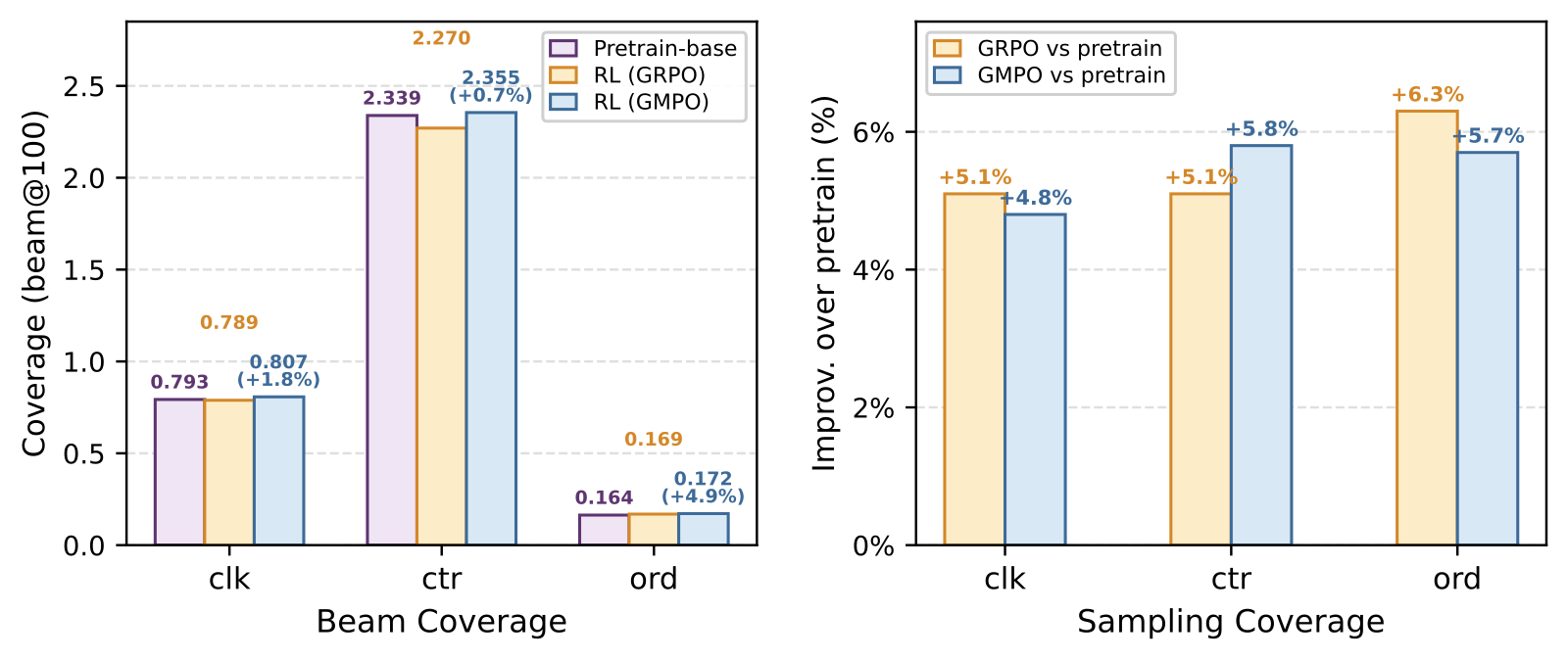
If candidates are not taken as the top scores by beam search but sampled randomly from the model's probabilities and then evaluated, GRPO and GMPO show almost no difference and both clearly beat the pretrained model; they only separate under beam search. The authors believe the randomness of sampling keeps a group of results diverse and masks the concentration of probability, while beam search deterministically takes the top-scoring batch of sequences, which reveals the concentration. Online decoding uses beam search, so the authors conclude that looking only at sampling evaluation would overstate the online gains of reinforcement learning.
Why does TS-GEAR lead by more than 30% at 20 km but barely at 5 km?
The offline evaluation data are 12 days of Taobao Shangou search ad logs, about 0.1 billion users and 4.8 million merchants, with the last day used for testing. TIGER represents a plain SID plus post-hoc distance filtering, GNPR and OneLoc are soft-signal schemes, and the three baselines use the same data, model size and beam configuration.
HitRate@N simulates the online pipeline: walk the beam in order, keep only deduplicated merchants within the radius, up to N of them, and count a hit if a merchant the user actually clicked is among them; the table below writes it as HR. All models filter by distance first and then truncate to N. So the HitRate gap does not come from anyone showing more shops outside the radius; it reflects how many candidates within the radius survive and how good their order is.
| Delivery radius | OneLoc HR@50 | TS-GEAR HR@50 | Relative gain |
|---|---|---|---|
| 5 km | 0.7778 | 0.7869 | +1.2% |
| 10 km | 0.7092 | 0.8090 | +14.1% |
| 20 km (online radius) | 0.5929 | 0.8080 | +36.3% |
This table answers where the gain comes from: the larger the radius, the larger the gap. The authors explain that within 5 km there are few reachable merchants, the top 50 reachable candidates already cover many of them, and all models approach saturation. As the radius grows, the reachable set grows, and the task becomes picking, from a larger set, the merchants the user will click.
Illustration: if there are only 60 merchants within 5 km, taking the top 50 nearly lists them all, and every model does about the same. Within 20 km there are 800, the top 50 are only one sixteenth, and the model must pick from 800 the ones the user will click, so the difference in how many beam slots go to reachable merchants shows.
ValidRate@N (called validity below) does no distance filtering and simply measures what fraction of the top N candidates fall within the radius. At 20 km, 95.8% of TS-GEAR's top 50 candidates fall within the radius versus 35.4% for OneLoc; for the top 300 candidates, the two are 93.0% and 29.3%. This shows that 60% to 70% of OneLoc's candidates are spent on merchants outside the radius, and TS-GEAR takes those slots back.
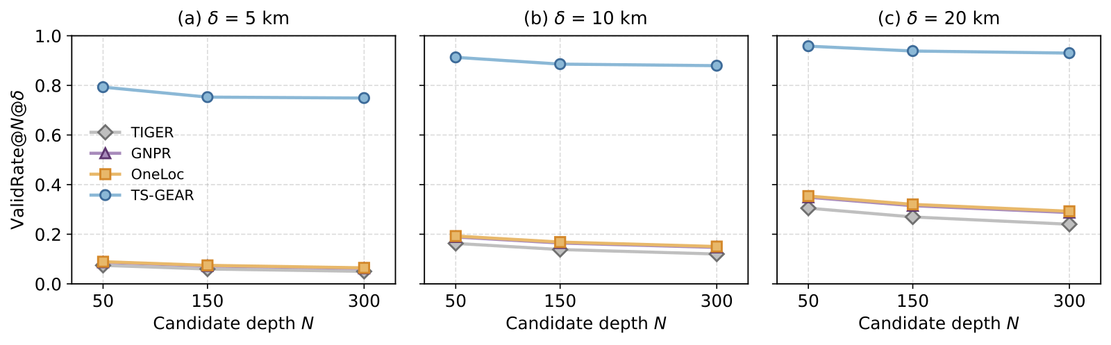
At 20 km, the gains over OneLoc on HR@50, HR@150 and HR@300 are 36.3%, 17.4% and 11.5% respectively. This shows that the fewer candidate slots there are (the smaller N is), the larger the gain from giving slots to merchants within the radius.
On the public Foursquare check-in data (New York and Tokyo subsets), TS-GEAR still ranks first, with HitRate 3.1% to 6.0% above OneLoc. These data have no delivery radius, and the query is only a placeholder (no real search terms, a default value is filled in), so the 3×3 grid constraint hardly applies. This shows that the trend of stronger geographic modeling giving better retrieval holds on another dataset too, while the 30%-plus margin appears in a setting with a delivery radius.
Removing which component makes HR@50 drop the most?
| Ablation variant | HR@50, 5 km | HR@50, 10 km | HR@50, 20 km |
|---|---|---|---|
| Full model | 0.7869 | 0.8090 | 0.8080 |
| Without Query Fusion | 0.7865 | 0.8092 | 0.8080 |
| Without User-Geo Gate | 0.7773 | 0.7961 | 0.7934 |
| Without Query-Geo Target Attention | 0.7661 | 0.7836 | 0.7820 |
| Without geographic prefix | 0.7794 | 0.7111 | 0.5947 |
| Without geographic prefix and User-Geo Gate | 0.7819 | 0.7124 | 0.5960 |
| Reference: OneLoc | 0.7778 | 0.7092 | 0.5929 |
Without the geographic prefix, HR@50 at 10 km and 20 km falls back to OneLoc's level, while 5 km barely moves. This shows that most of the lead at large radii is due to the geographic prefix.
Once the geographic prefix is removed, also removing User-Geo Gate is slightly better than keeping the gate, 0.5960 versus 0.5947 at 20 km. The authors explain that the gate can only reorder cells the prefix has already restricted to be reachable; without that premise, it only adds noise to the decoding order over the whole ID space. This shows that the geographic prefix and the gate must be used together, and their contributions cannot simply be added up.
With the prefix kept and only the gate removed, HR@50 at 20 km drops by 1.46 percentage points, and the larger the radius and the more reachable merchants there are, the more it drops. The authors see the two components as a division of labor: the geographic prefix decides which cells are allowed, and the gate decides which cell to write first. Removing Query-Geo Target Attention hurts more, 2.60 percentage points at 20 km, and varies relatively little with the radius. The authors take this to mean that Query-Geo Target Attention works on the interest representation, because whether A wants fresh groceries or hot food has nothing to do with the radius. Query Fusion makes a difference of no more than 0.05 percentage points on the full population, because it is a fallback for users with sparse history and its effect is diluted over all traffic.
The authors also give an argument. If one decoded plain SIDs and directly masked candidates outside the radius, validity could also approach 100%, but the model's probability distribution never learned geography, so the surviving candidates would still be ordered without regard to location. The closest evidence is the gate experiment above: with the 3×3 grid constraint unchanged and only the gate removed, HR@50 at 5 km to 20 km still drops by 0.96 to 1.46 percentage points. This shows that once the grid constraint is fixed, the gate still improves hit rate, which may involve changes both in the number of candidates within the radius and in their order. Fresh-grocery shops and hot-food shops near A's home are both within the radius, and only ranking the fresh-grocery shops first turns into a hit.
How much did it gain online, and who bears the cost?
The deployed model is the 0.1B tier. The authors tried three tiers, 0.05B, 0.1B and 0.5B: HitRate rises roughly linearly with capacity while validity stays essentially flat, from which the authors conclude that validity is mainly determined by the prefix constraint. The 0.1B tier was chosen to meet online latency requirements: on the A10 GPUs used for deployment, the latency budget is 70 ms. The 3×3 grid also saves compute here, since online serving skips generating the first two geographic tokens and reuses the KV cache.
Online, TS-GEAR is one incremental retrieval channel running in parallel with existing channels such as keyword and vector retrieval, and the results enter ad ranking and bidding together. The treatment group with this channel added took 20% of traffic for 7 consecutive days; compared with the control group, ad impressions rose 3.8% and ad revenue rose 4.2%, both at p<0.01. This shows that on a pipeline that already has multiple retrieval channels, adding this one still increases revenue. These numbers are the effect of the whole channel and are not broken down into the separate online contributions of the geographic prefix, Query-Geo Target Attention or GMPO. TS-GEAR is now fully deployed and serves more than 150 million search requests per day.
The authors also describe the costs themselves. Because decoding is restricted to the 3×3 grid and the reward is dominated by business value, exposure concentrates on nearby merchants with high historical conversion. Newly onboarded merchants and merchants in remote areas appear less often among the candidates and have to spend more on ads to get comparable exposure.
Back to A's search. The 3×3 grid first keeps merchants in other cities out of the beam, and the third geographic token steers slots toward the small cells near A's home. After past behaviors are reweighted by location and query, last Saturday's beef brisket purchase at home gets the largest weight, and GMPO makes training stop rewarding the same shop repeated. All of these steps happen before the ID is fully written or during training, and at the online 20 km radius, fewer than 5% of the top 50 candidates still need to be removed by distance filtering.
How did this read for you?
Hoot made a note. Thanks for the feedback.

One tap, no sign-in; tap again to undo. Only anonymous counts are kept, never who you are.
Related papersMore from Paper Daily
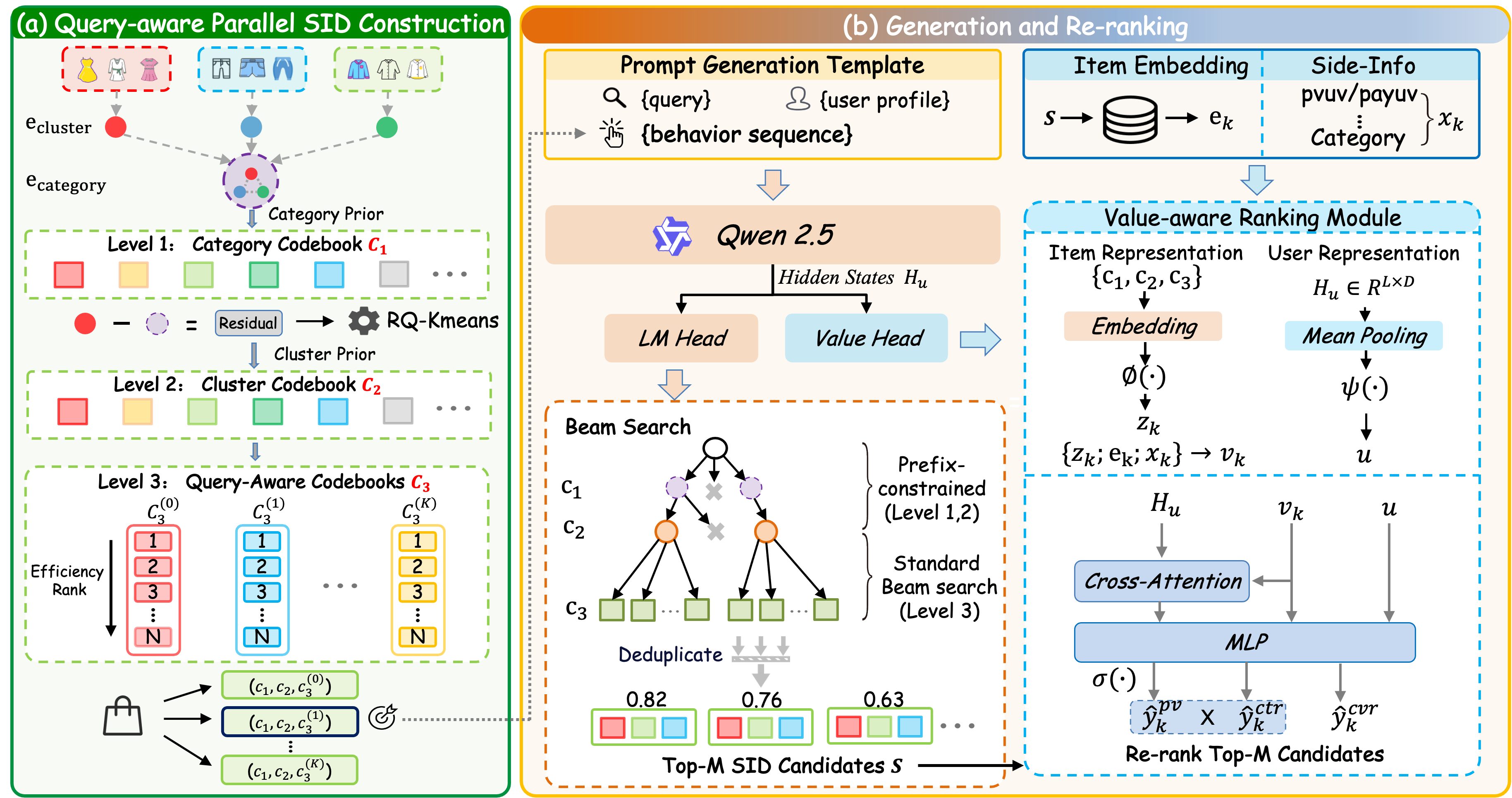 Generative · 2026-07-23TSGR: Taobao Search Generative RetrievalDeep dive: TSGR: Taobao Search Generative Retrieval.
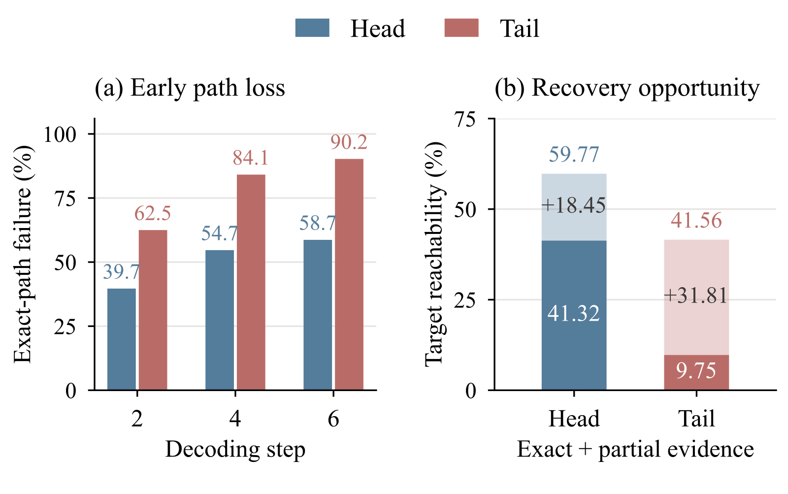 Generative · 2026-11-16ReSID: Rethinking Long-Tail Retrieval in Generative Recommendation through Item ReachabilityGenerative recommendation encodes each item as a string of Semantic ID tokens and generates them one position at a time with beam search, and cold long-tail items are hard to retrieve this way. The authors take apart the whole chain from encoding through decoding to matching and find that tail items are mostly lost early in decoding: on Amazon Industrial, 62.5% of tail targets have already fallen…
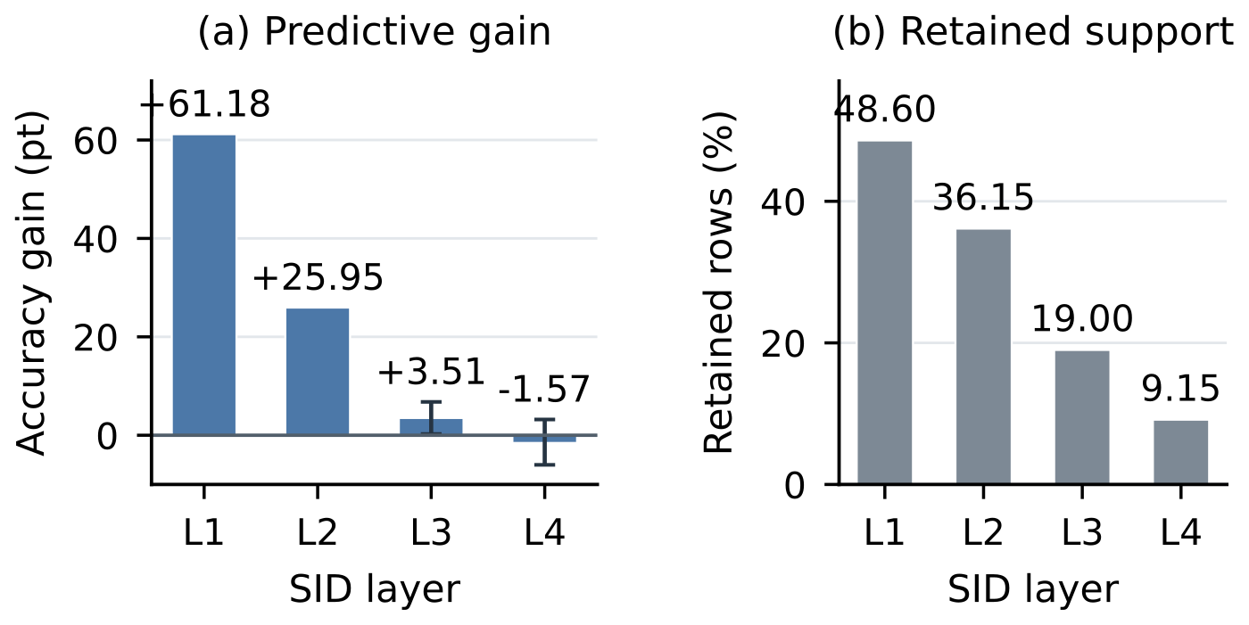 Generative · 2026-11-05ReuseGR: Offline--Online Decoupled Generative Retrieval via Adaptive Prefix ReuseTeams putting generative retrieval into production should read this: it shows how to reuse large-model compute per query while leaving personalization to a small online model, and it is backed by an online A/B test. The same query is searched by many people every day, so generating a full Semantic ID from scratch for each request repeats work. ReuseGR splits the job in two. Offline, a large model…
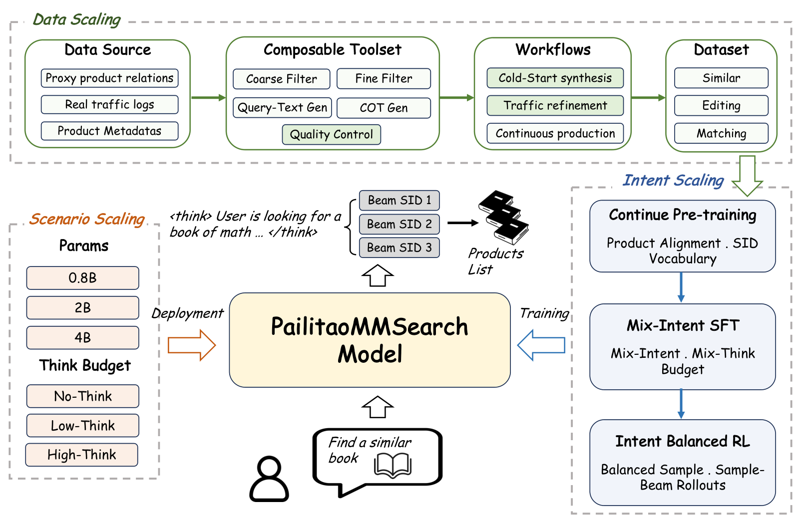 Generative · 2026-10-29PailitaoMMSearch2.0 Technical Report: Scaling Generative Retrieval to Unified End-to-End Multimodal SearchIn Taobao's Pailitao, a user may photograph a shirt and ask for shorts to match it, which calls for a complementary item rather than a duplicate. The usual pipeline classifies intent first and routes to separate retrieval channels, so one wrong step breaks everything after it. Alibaba's report lets a 2B vision-language model read the raw image and instruction and generate product Semantic IDs dir…
 Personalization · 2026-11-06From Waste to Discovery: Recycling High-Scored Unexposed Candidates in Taobao Feed RecommendationRanking already scores many candidates that never reach the screen. This work reuses the high-scoring part of those results to help users encounter additional categories. It accumulates these candidates per user over a month, keeps categories absent from recent exposure, and adds the results to recall. In Taobao feed experiments, new categories actually exposed to users increased by 3.47% and com…
 Generative · 2026-11-17RecMem: Recurrent Memory Compression for Long-Sequence Generative RecommendationOnce a generative recommender feeds a user's long history straight into the model, compute and memory grow with history length, and long interaction sequences quickly become slow and expensive. The authors compress history segment by segment into a fixed number of memory slots, and the decoder uses a fixed-length context that no longer expands as the history grows. On a long-sequence benchmark fr…
 Generative · 2026-11-16TriGen: A Generative Paradigm for Trigger-Induced RecommendationE-commerce has a common kind of recommendation: a user clicks an item in the main feed and lands at once in a feed built around that item. The recommendations must follow the intent of that click without throwing away the user's long-term taste. Generative recommendation by default just continues the user's history with more SIDs, so one click is easily diluted in a long history, while traditiona…
 Generative · 2026-11-02PFA: Attention Can Be Progressively Focused in Long-Sequence Generative RecommendationThe authors at Alibaba found that when a generative recommender decodes with beam search, attention concentrates on a few past behaviors as decoding proceeds, and which behaviors matter stays largely the same from step to step. Building on this, PFA picks the important history once for the whole decode, instead of having every beam pick it again at every step. It attends to the full history as us…
Discussion
Add experiment details, reproduction notes or a different take. Requires a GitHub sign-in.
Loading the discussion…