Contents · 9 sections
1What problem does it solve?2Overview: score with the mean, weight with the variance3Step 1: turn the score into a Gaussian4Step 2: the PPR loss and two constraints5Step 3: weight pairs by variance6What the experiments show7Limitations as I see them8How a recommendation team could try it9Conclusion and assessmentSHARE

Teams working on multi-objective fusion ranking for short video or feeds should read this, especially those that have already replaced hand-tuned fusion formulas with an end-to-end model. This Kuaishou paper proposes UAME (Uncertainty-Aware end-to-end Multi-objective Ensemble ranking). The core idea in one sentence: besides scoring each video, the ranking model also outputs a variance that expresses how much the behavioral objectives disagree about this video's rank, and video pairs with high variance get more weight in training. Offline, on the EMER base (a widely deployed end-to-end fusion ranking model), the GAUC of the follow prediction pwtr rises from 0.684 to 0.724 (Table 1). Online, two groups with 5% of traffic each ran for 7 days: long views rose +1.614% and +1.126%, while 7-day retention rose only +0.009% and +0.015% (Table 2). In my view the idea worth borrowing is how cheap it is: no extra labels, only the mean is used for online scoring, and inference cost does not grow. However, the offline evaluation leaves the data scale unstated, and one ablation scores below the untouched base, so it is not clear which part the gain comes from.
What problem does it solve?
Ranking in short-video recommendation usually has two steps. First, a multi-task model predicts a set of pxtr scores for each candidate video; the paper uses 8 of them: click pctr, watch time pvtr, long view plvtr, complete view pcpr, like pltr, follow pwtr, comment pcmtr, and share pftr. Second, these scores are fused into one final score. Early systems used handwritten formulas (weighted sums or products). Later methods such as EMER and EASQ (a method that adds questionnaire satisfaction feedback as supervision in fusion ranking) learn the fusion directly with a deep model, collectively called end-to-end multi-objective ensemble ranking.
How are these models trained? There is no label for true user satisfaction, so the pxtr scores serve as proxies. For any two candidate videos and , the -th pxtr yields a pairwise label: 1 if , otherwise 0. With pxtr scores there are pairwise labels, and the model computes a pairwise ranking loss on each one with equal weight.
The paper argues the problem lies here. Different pxtr scores often disagree about the same pair: one video has a high click rate but is rarely finished, another has a low click rate but many likes. Under equal weighting, pairs on which all pxtr scores agree are easy to learn and dominate the gradient. Pairs with conflicting opinions are the ones that actually decide fusion quality, yet they get averaged away. In addition, the model outputs a single deterministic score per video, which amounts to assuming one score can satisfy all the conflicting objectives at once.
A toy example runs through the article. One request has 5 candidate videos, and here we look at three of them and their ranks under three pxtr scores:
| Video (toy) | pctr rank | pvtr rank | pltr rank | Rank std |
|---|---|---|---|---|
| A | 1 | 1 | 2 | 0.47 |
| B | 2 | 5 | 1 | 1.70 |
| C | 5 | 4 | 5 | 0.47 |
The ranks of A and C are largely consistent across objectives, and A clearly belongs ahead of C. B is near the top on clicks and likes but near the bottom on watch time, so the objectives disagree about whether it should come before A or C. UAME wants the model to know by itself that B is "controversial" and to pay more attention to it during training.
Overview: score with the mean, weight with the variance
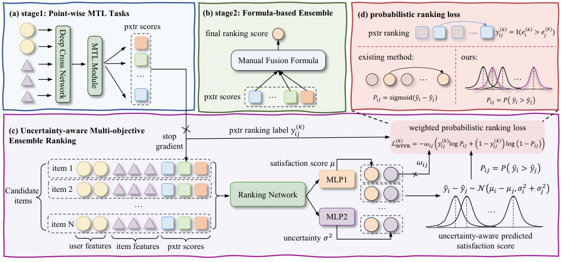
The method has four parts:
| Module | Input | Output | Role |
|---|---|---|---|
| Two-branch output layer | User features, video features, pxtr scores | and per video | Give uncertainty besides the score |
| PPR loss | and of two videos, pairwise label of the -th pxtr | One pairwise cross-entropy term per pxtr | Learn variance together with ranking |
| Auxiliary constraint | Each video's rank std across pxtr scores | A pairwise logistic loss | Make variance actually track objective conflict |
| Adaptive weighting | Sum of the pair's variances | Weight | Learn more from high-conflict pairs |
At serving time only is used for ranking, and the variance branch takes no part in scoring (Appendix B), so inference cost equals that of the base. The variance only matters during training, where it decides how much each pair is learned.
Step 1: turn the score into a Gaussian
Why output a variance? A single deterministic score cannot express that a video is judged very differently under different objectives. After the original ranking network, UAME attaches two two-layer MLPs that share features. One outputs the satisfaction score and the other outputs (exponentiated to get a non-negative variance), and the video's score is treated as a random variable:
Assuming the two videos' scores are conditionally independent, the difference is also Gaussian, so the probability that should rank ahead of has a closed form:
is the standard normal cumulative distribution function. A quick calculation: if A and C differ by 0.5 in mean and their variances sum to 0.25, the square root is 0.5 and . If A and B also differ by 0.5 in mean but B has a large variance, so the sum is 1, then . With the same mean gap, a larger variance means the model is less sure about the order.
Step 2: the PPR loss and two constraints
With , each pxtr's pairwise label can be plugged into a cross-entropy, which the paper calls the PPR (Probabilistic Pairwise Ranking) loss. It moves both the mean and the variance. When the label is 1 (this pxtr prefers ) and the model ranks the pair correctly, it widens and shrinks the variance, pushing toward 1. When the label is 0 the direction flips and is pushed toward 0. When it ranks a pair wrongly, besides moving the means in the right direction it also raises the variance, making the judgment "less sure". So if a pair is pulled in opposite directions by different pxtr scores, its variance naturally grows. Figure 2 draws exactly this: A and C receive gradients in a consistent direction and their distributions are sharp and narrow, while B receives conflicting gradients and its distribution widens.
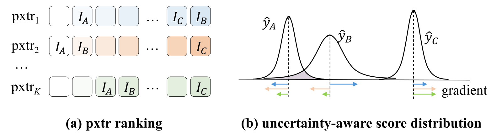
There is a shortcut here: the model could make every variance large so that every sits near 0.5, keeping the loss moderate without learning to rank. To block this, the authors add a regularizer that penalizes with coefficient .
Variance learned from PPR alone is only indirectly supervised and need not correspond to objective conflict. So the authors add an auxiliary constraint. For each video they compute the standard deviation of its ranks across the pxtr scores as its conflict level. They then pick pairs where the conflict of is clearly higher than that of , require , and train this with a pairwise logistic loss with coefficient . In the toy table, B's std of 1.70 is far above A's 0.47, so this pair would enter the auxiliary training set. The paper words this filter only as "significantly higher conflict".
Step 3: weight pairs by variance
Why can variance serve as a weight? The authors define a pair's combined uncertainty as the sum of the two variances, . They apply min-max normalization over all pairs in the current batch and multiply by a scaling coefficient :
The total loss is the sum of the weighted PPR losses, plus times the regularizer and times the auxiliary loss.
A quick calculation: suppose the batch's ranges from 0.25 to 2.25 and the A–B pair has , so its weight is . If the A–C pair happens to be the batch minimum, its weight is 0. By this formula, the pair with the smallest variance in the batch drops out of the ranking loss entirely, and easy pairs where the objectives agree are heavily down-weighted. This follows directly from the formula, and the authors do not discuss its effect specifically.
On the theory side, the authors split the true ranking risk into a surrogate risk plus a surrogate bias. They prove that the surrogate bias of a single pair is proportional to the gap between the true label and the average of the pxtr labels (Lemma 3.1). Adding an empirical assumption, that the sum of variances grows in expectation with pxtr conflict (Assumption 2), yields that bias and variance are positively correlated in expectation (Proposition 3.2). This means the theoretical basis for the weighting rests mainly on Assumption 2, which is supported by the later questionnaire experiment.
What the experiments show
The offline experiments use real Kuaishou data, the main metric is GAUC on each pxtr, and the bases are EMER and EASQ. There are three baselines: RankDist, which uses variance to adjust scores at inference; EBRank, which explores with empirical Bayes and an upper confidence bound; and ANSL (a method that weights samples automatically by loss size). A few columns from Table 1:
| Base | Method | pctr | pvtr | plvtr | pltr | pwtr |
|---|---|---|---|---|---|---|
| EMER | Base Model | 0.706 | 0.667 | 0.731 | 0.688 | 0.684 |
| EMER | ANSL | 0.666 | 0.715 | 0.670 | 0.669 | 0.709 |
| EMER | UAME | 0.715 | 0.699 | 0.735 | 0.712 | 0.724 |
| EASQ | Base Model | 0.672 | 0.598 | 0.668 | 0.682 | 0.661 |
| EASQ | ANSL | 0.670 | 0.636 | 0.677 | 0.712 | 0.666 |
| EASQ | UAME | 0.734 | 0.669 | 0.763 | 0.684 | 0.675 |
On EMER, UAME is best on 7 of the 8 pxtr scores and trails ANSL only on pvtr. ANSL is higher on pvtr but clearly below the base on pctr and plvtr. This suggests that weighting by loss size alone helps one objective at the expense of others, while weighting by objective conflict is more balanced. On EASQ, UAME lifts plvtr from 0.668 to 0.763, but its pltr is below ANSL.
The online A/B test ran for 7 days, with two groups each taking 5% of main-feed traffic, one compared against EMER and one against EASQ, and every metric had a p-value below 0.005. Gains in long views, likes, follows and shares fall between 0.6% and 1.6%, while App stay time rose only +0.050% and +0.074%. This means the gains show up mainly in engagement and long views, with little effect on overall time spent and retention.
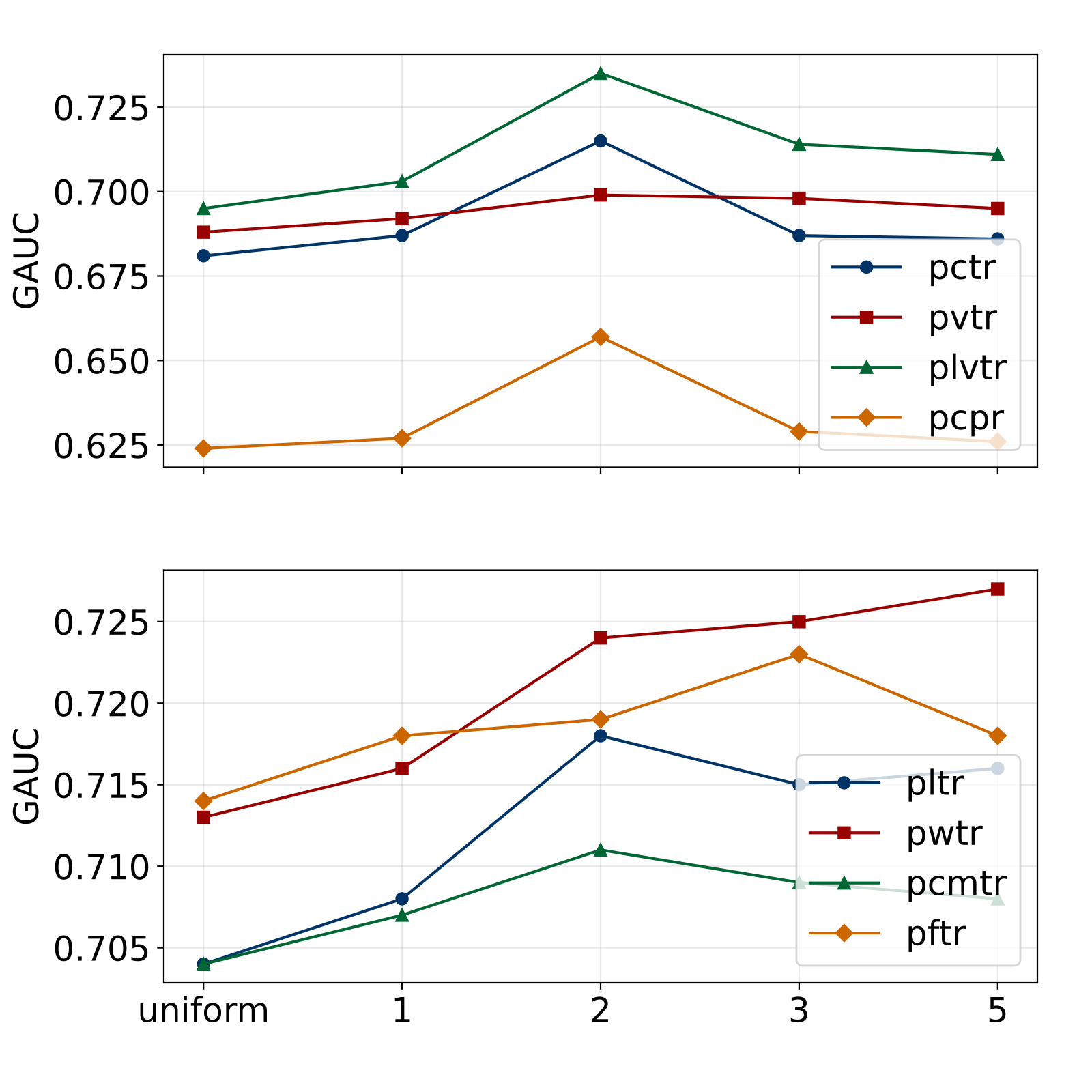
Figure 3 doubles as the ablation: setting to 0, setting to 0, and setting all weights to 1 all do worse than the full version. Figure 3(c) deserves attention. With all weights equal to 1, pctr is about 0.681 and pcpr about 0.624, both below the EMER base's 0.706 and 0.640 in Table 1. Note that this setting still keeps the variance regularizer and the auxiliary constraint and only removes the weighting. So it shows that adaptive weighting contributes when the other components are present, but it cannot isolate the effect of the PPR loss, nor fix each component's share of the gain.
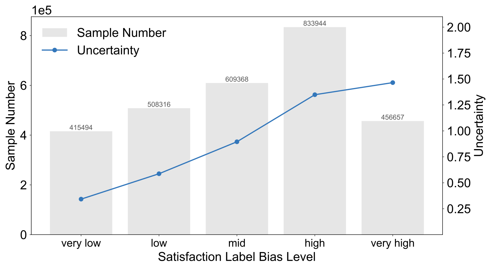
Finally, the authors use questionnaire satisfaction from EASQ as an approximate ground truth. In Table 3, UAME raises NDCG@5 from 0.3753 to 0.4080 and HR@5 from 0.8192 to 0.9063. Label bias is computed per pair: the questionnaire gives a pairwise label for which video in the pair satisfies the user more, the average of the pxtr pairwise labels is subtracted, and the absolute value is taken (Appendix C). On 3 million samples, the Pearson correlation between the learned uncertainty and this bias is 0.65 and the Spearman correlation is 0.67. Appendix Figure 4 splits samples into five bins by bias, and the mean variance rises monotonically with bias. This indicates that variance does, to some extent, reflect the mismatch between behavioral labels and true satisfaction.
Limitations as I see them
First, basic information about the offline evaluation is thin. The dataset is described only as coming from a platform with hundreds of millions of daily active users. Sample size, time span and the train-test split are all left out. Which real behavior the GAUC is computed against is also not written down. In Table 1, the EASQ base scores only 0.598 on pvtr, nearly 7 points below the EMER base, and that gap between the two bases itself needs explaining.
Second, the source of the gain is unclear. In Figure 3(c) the unweighted version is about 2.5 points below the base on pctr, which suggests that without weighting, the PPR loss plus the two constraints is not necessarily better than the base; there is no control that swaps in only the PPR loss without the constraints. Also, pwtr is still rising at ; the authors chose based on overall performance, and the optimal value differs across objectives.
Third, the online gains are small, and the questionnaire validation was done only on EASQ. A 7-day retention gain of +0.009% and +0.015% is significant but of limited business meaning. The questionnaire experiment is the only evidence that variance reflects label bias, and no such check was run on EMER.
How a recommendation team could try it
- First confirm offline whether objective conflict is serious. On the training samples of the existing fusion model, compute each candidate's rank std across pxtr scores and see what share of samples are high-conflict. If the vast majority of samples have consistent objectives, there is little room for this method.
- Then add the variance branch and the PPR loss, without weighting at first. Compare GAUC with the original model to see whether the unweighted version loses points, as Figure 3(c) hints it may.
- Then add min-max weighting by variance, sweep a few values starting from , and watch GAUC on each pxtr rather than only the average.
- If questionnaire or human satisfaction labels are available, reproduce the variance–bias correlation check, which is the most direct evidence of whether the variance is meaningful.
Conclusion and assessment
The key takeaway: in multi-objective fusion, the samples on which objectives conflict carry the most information, and the model can find them through its own learned variance without extra labeling.
| Dimension | Assessment |
|---|---|
| Problem importance | High. End-to-end fusion ranking is now mainstream in short-video recommendation, and the gap between proxy labels and true satisfaction is a common problem |
| Novelty | Medium. Gaussian scores and probabilistic pairwise losses are existing ideas; the novelty is using variance for sample-level weighting and linking it to label bias |
| Evidence | Medium. Two bases, an online A/B test and a questionnaire correlation are all present, but the data scale is unstated and the unweighted ablation falls below the base |
| Engineering cost | Low. Only one output branch and a few loss terms are added, and serving is unchanged |
| Worth trying? | Yes, provided your data has enough objective conflict; first confirm, as in step 2 above, that the unweighted version does not lose points |
How did this read for you?
Hoot made a note. Thanks for the feedback.

One tap, no sign-in; tap again to undo. Only anonymous counts are kept, never who you are.
Related papersMore from Paper Daily
 Retrieval · 2026-08-03SaFRO: Satisfaction-Aware Fusion via Dual-Relative Policy Optimization for Short-Video SearchDeep dive: SaFRO: Satisfaction-Aware Fusion via Dual-Relative Policy Optimization for Short-Video Search.
 Personalization · 2026-11-17RACE: Ranking-Uncertainty Aware Capacity-Adaptive Customization for Efficient Sequential RecommendationOn-device sequential recommenders often compress every request with the same ratio, so simple interests waste compute and complex ones do not get enough capacity. Pruning and decomposition usually freeze the model and the input at a fixed size, and cannot adjust capacity to how hard the current behavior sequence is. The authors estimate difficulty from how stable the model's current ranking is, t…
 Personalization · 2026-10-19RecSoup: Efficient Model Merging Approach for Controllable Multi-Objective RecommendationRecSoup makes accuracy–diversity trade-offs adjustable by reusing objective-specific checkpoints. It prunes task-vector updates and learns preference-dependent merge coefficients. Parameter construction was about 165–228 times faster than a hypernetwork across three benchmarks.
 Generative · 2026-06-05Bridging Short Videos and Live Streams: Reasoning-Guided Multimodal LLMs for Cross-Domain Representation LearningDeep dive: Bridging Short Videos and Live Streams: Reasoning-Guided Multimodal LLMs for Cross-Domain Representation Learning.
 Personalization · 2026-11-03Lightweight Ranking Heads: Accelerating Multi-Task Experimentation in Production Recommender SystemsThe bigger a multi-task ranking model gets, the slower it becomes to add a new prediction target. YouTube's answer keeps the new target out of the main model and makes it a small prediction head on top of the shared layers (the paper calls it a Light Head). It only reads the shared layers' output, sends no gradient down, and is reset at the start of every training run, and every ranking model rea…
 Personalization · 2026-09-10Task-Blind No MORE: Multi-Task Information Flow in Unified Ranking BackbonesDeep dive: Task-Blind No MORE: Multi-Task Information Flow in Unified Ranking Backbones.
 Personalization · 2026-11-16Measuring, Revealing and Mitigating Harmful Content Propagation in Recommender SystemsRecommenders chase user interest, and few ask whether what they push is harmful. The authors sampled 100 recommendation lists produced by BERT4Rec and found that nearly half of the items contained gender discrimination, misinformation, or offensive language. They had an LLM label the items in three news and advertising datasets as harmful or healthy with a reason, then had humans review the label…
 Personalization · 2026-10-21FLMNet: Self-Ensemble Distillation from Masks to Seeds for Single-Tower CTR PredictionCTR self-distillation can be replaced with a computable disagreement penalty. FLMNet keeps gates on clean inputs and distills independently trained towers into one serving model. The distilled model reaches 0.8169 AUC on Criteo.
Discussion
Add experiment details, reproduction notes or a different take. Requires a GitHub sign-in.
Loading the discussion…