Contents · 10 sections
1What problem is it solving?2The big picture first3Change one: aggregate features by averaging instead of summing4Change two: compress the ad side into one token and spend the saved compute on the model5Change three: add domain information like a positional encoding6Scaling curve and main comparisons7How it fits into 40 ms in production8Limitations as I see them9How a retrieval team could try it10VerdictSHARE

Retrieval teams should read this, especially those already doing retrieval with "a scoring model plus a graph index" who want to make the model bigger. The problem it addresses: the ranking stage now has plenty of "bigger model, better results" evidence, but retrieval has very little, because retrieval must pick a few thousand items out of tens of millions within tens of milliseconds, every visited candidate passes through the model, and compute is multiplied by the number of candidates. The core idea in one sentence: first put input features on the same scale, then squeeze all ad-side features into a single token to save compute, and spend the saved compute on a wider, deeper Transformer. Key numbers: raising per-candidate compute from about 0.14 to 1.91 MFLOPs (millions of floating-point operations) lifts Recall@2000 on the industrial data from 0.464 to 0.657; a month on 5% of online traffic raised platform revenue by 2.53%, with P99 latency still under 40 ms, the same as the old system.
What problem is it solving?
Start with an illustrative scenario. A user opens a Taobao page, and the display ads system must pick 2,000 candidates out of 52M ads to hand to the ranking stage. Alibaba's retrieval is not a two-tower model but model-based retrieval: the ads are pre-built into an HNSW graph (a layered nearest-neighbour search graph), and a scoring model walks the graph with beam search, actually scoring only about 40K ads per request, roughly 0.08% of the corpus.
A two-tower model can only score with the inner product of a user vector and an ad vector, so user and ad features cannot interact at a fine grain; model-based retrieval can use an arbitrarily complex scoring network, at the price of one forward pass per visited candidate. So the expensive part here is not the user side but the compute spent on each candidate, which is multiplied 40,000 times.
To replace the scoring model with a larger Transformer in this setting, the authors list three obstacles:
| Obstacle | What it looks like | TransRetrieval's answer |
|---|---|---|
| Features on different scales | After summing, user-side multi-value features (say, dozens of past categories) produce vectors up to 10× longer than ad-side ones | Replace the sum with a weighted average |
| Candidate-side compute too expensive | Every feature of every ad is a token, so compute grows linearly with feature count and is then multiplied by 40K | Compress ad-side features into 1 token with an MLP |
| Multiple business domains | Homepage, search, detail page and so on have different distributions; separate models double the cost and small domains lack data | Learn one vector per domain and add it to every token, like a positional encoding |
All three changes use only standard operators and need no new infrastructure. The sections below explain why each is done and how much it helps.
The big picture first
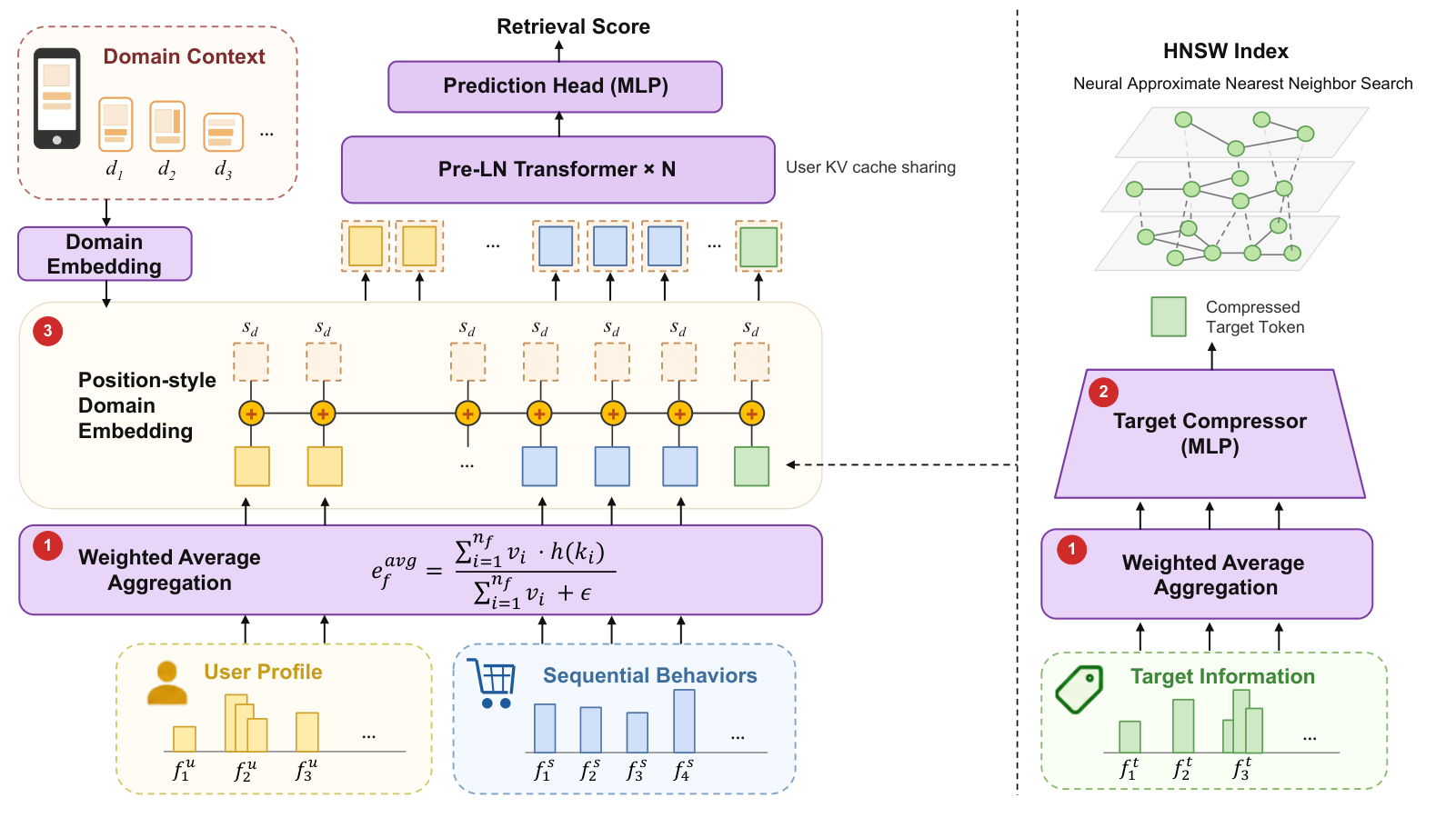
The computation for one request:
| Step | What happens | How many times per request |
|---|---|---|
| 1. Encode the user side | User features and the behaviour sequence are aggregated into tokens, the domain vector is added, and each layer's KV is computed and cached | Once |
| 2. Compress the ad side | Ad features are aggregated and compressed by the MLP into 1 token (can be precomputed offline) | Precomputed, refreshed near-line when features change |
| 3. Score candidates | The ad token acts as the query, attends to the cached user KV, then goes through the prediction head | About 40K times |
| 4. Graph search | Beam search on the HNSW graph by score, keeping the top 2,000 | Interleaved with scoring |
Change one: aggregate features by averaging instead of summing
A feature field in recommendation often holds several values; "recently clicked categories" might have dozens, each with a weight. The usual approach adds up the values' embeddings by weight. The problem is that the summed vector grows longer as the number of values grows. A quick hand calculation (illustrative): 100 embeddings of length 1 pointing in unrelated directions sum to a vector of length about √100=10; if they all point the same way, the length is 100. Many ad-side fields have just one value, so their length is 1. The authors measured user-side tokens up to 10× longer than ad-side ones.
Why is this harmful? An attention score is the dot product of query and key, so a longer key gets a larger score. Suppose two keys are equally similar in direction to the query and both originally give a dot product of 0.5; stretch one of them 10× and its dot product becomes 5, so after softmax it takes e^5/(e^5+e^0.5)≈0.99 of the weight and the other is almost ignored. The authors see this as the reason stacking Transformer layers on recommendation features stops helping.
The fix is to divide by the sum of weights:
Now, however many values a field has, the result is never longer than a single embedding. It needs no learned parameters and no statistics.
Ablation (64D-5L configuration, industrial data, Recall@2000):
| Aggregation | Overall Recall@2000 |
|---|---|
| Weighted average (this paper) | 0.618 |
| Weighted sum | 0.608 |
| Sum followed by LayerNorm | 0.593 |
| Max pooling | 0.571 |
This shows averaging is indeed best, but only 1.0 point above summing, which looks small for something the abstract calls the "key enabler". Two more points deserve attention. First, averaging only caps the length; it does not make fields equally long: averaging 100 vectors in unrelated directions actually shrinks the length to about 0.1, a case the authors do not discuss. Second, the model is a Pre-LN Transformer, which applies LayerNorm before attention in every layer and should therefore equalise token lengths; the "long tokens hog attention" explanation does not fully fit the architecture. A more likely route is the scale difference in the residual stream, but the paper does not analyse it.
Change two: compress the ad side into one token and spend the saved compute on the model
The authors give a formula for the total compute of scoring all candidates in one request:
D is the hidden size, the number of scored candidates, the tokens per candidate, the user-side tokens, and the number of layers. D and the layer count are what we want to grow, the candidate count has already been cut to 0.08% by HNSW, and is the only thing left to reduce. So the authors concatenate all ad-side features and pass them through a three-layer MLP (widths 8D, 4D, D) into a single D-dimensional token.
The paper's tables report compute per candidate, which is this formula without , namely , and it can be used to check the numbers. The paper does not give directly; from 64D-3L with 8 tokens at 3.04 MFLOPs I back out of about 240 (my estimate). Plugging it back in:
| Configuration | Formula estimate (MFLOPs) | Reported | Recall@2000 |
|---|---|---|---|
| 64D-3L, 8 tokens | 4×64×8×(256+240)×3≈3.05 | 3.04 | 0.624 |
| 64D-3L, 4 tokens | about 1.52 | 1.55 | 0.615 |
| 64D-3L, 1 token | about 0.38 | 0.45 | 0.603 |
| 128D-5L, 1 token | 4×128×1×(512+240)×5≈1.92 | 1.91 | 0.657 |
The formula and the reported values largely agree; the extra ~0.07 at 1 token is presumably the compression MLP itself. The table shows the authors' reasoning: compressing to 1 token cuts compute by about 85% and costs 2.1 points of Recall, but spending the saved compute to grow the model from 64D-3L to 128D-5L still uses less compute than the small 8-token model (1.91 vs 3.04) and gains 3.3 points of Recall. At 40K candidates per request, 128D-5L spends about 76 GFLOPs per request on the candidate side (my estimate).
A further benefit is that the compressed token is itself a fixed-dimension vector that can be used directly to build the HNSW index. When ad features change, only the affected ads' tokens need recomputing near-line.
Change three: add domain information like a positional encoding
Alibaba display ads serves 4 business domains. If all data is mixed into one model, the model cannot tell which domain a request comes from; a common fix is to add a few "domain tokens" to the sequence, but each extra token adds attention cost. The authors instead learn one D-dimensional vector per domain and add it directly to every token, just like a positional encoding: the sequence length stays the same and all Transformer parameters are fully shared across domains.
| Approach (64D-3L, industrial data) | Overall Recall@2000 | User-side MFLOPs |
|---|---|---|
| Train each domain separately | 0.579 | 41.3 |
| Mixed training, no domain information | 0.265 | 41.3 |
| Mixed training, 1 domain token | 0.337 | 41.8 |
| Mixed training, 20 domain tokens | 0.452 | 49.8 |
| Mixed training, domain vector added to every token (this paper) | 0.603 | 41.3 |
This shows mixed training only pays off when the domain signal is strong enough: 1 token barely helps, repeating it 20 times helps clearly, and adding it to every token works best at no extra compute. Compared with per-domain training, domain B gains the most, from 0.539 to 0.590, while domain A only moves from 0.591 to 0.593.
One thing in this table is puzzling, though: mixed training with no domain information gets only 0.265, less than half the single-domain 0.579. All four domains are traffic from the same ad platform, so dropping this far just by mixing them is very unusual, and the paper does not explain why. Also, on the public KuaiRand data, on the sparsest domain, Tab 3 (only 0.13% of interactions), TransRetrieval scores 0.537, below HSTU's 0.611, so the claim that "small domains benefit from cross-domain transfer" does not always hold on public data.
Scaling curve and main comparisons
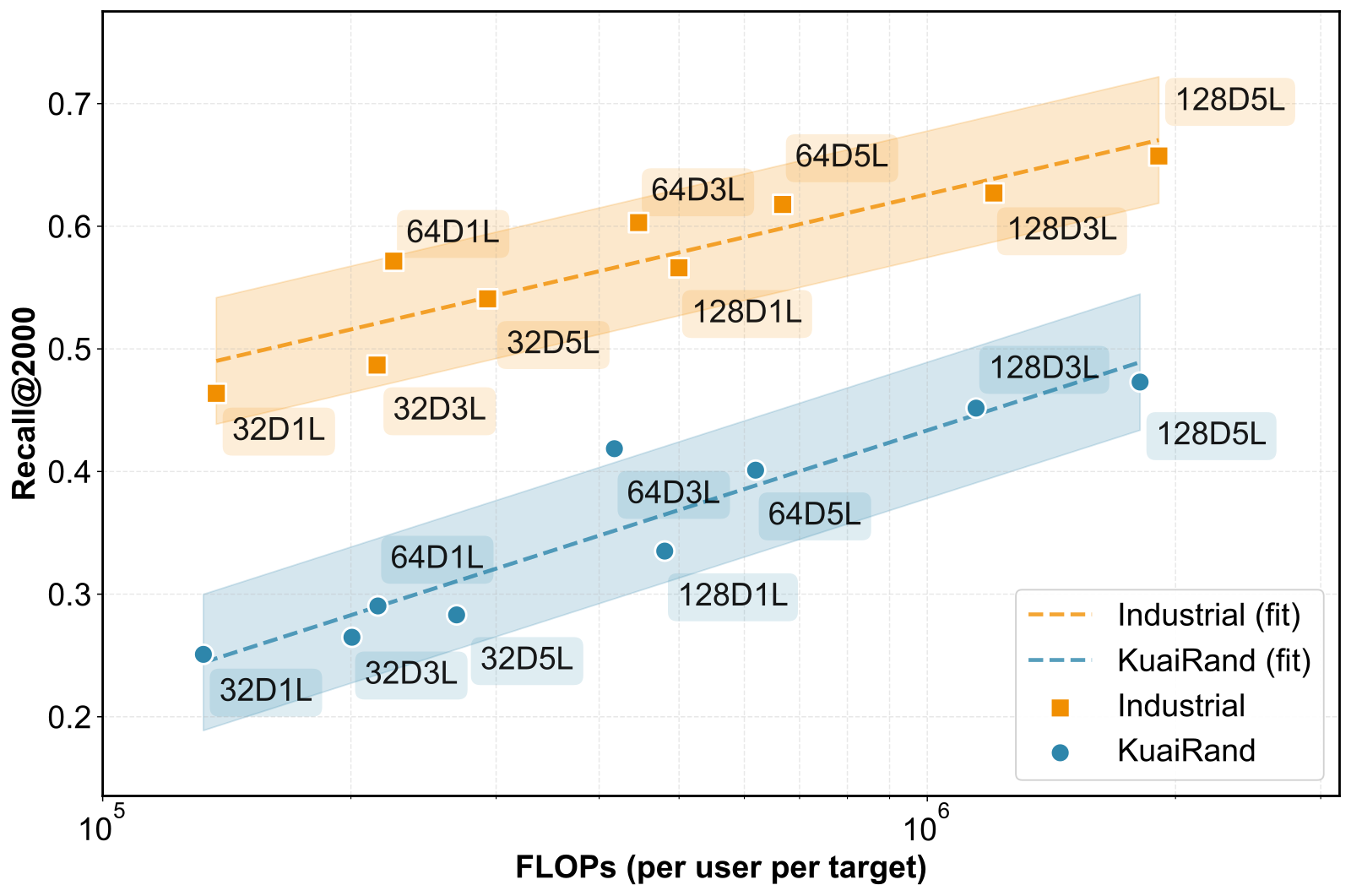
From 32D-1L to 128D-5L, industrial Recall@2000 rises from 0.464 to 0.657 and KuaiRand from 0.251 to 0.473, with log-linear fit R² of 0.82 and 0.88, showing the trend is stable overall but the points scatter noticeably. Against the baselines (industrial data, overall Recall@2000):
| Method | Recall@2000 | MFLOPs per candidate |
|---|---|---|
| Two-tower KuaiFormer-128D5L | 0.495 | 0.011 (amortised) |
| Previous production system | 0.576 | 0.69 |
| HSTU-128D5L | 0.527 | 1.72 |
| RankMixer-768D16T | 0.531 | 150.99 |
| TransRetrieval-64D3L | 0.603 | 0.45 |
| TransRetrieval-128D5L | 0.657 | 1.91 |
64D-3L uses 35% less compute than the production system and scores 2.7 points higher; 128D-5L beats RankMixer-768D16T, which uses nearly 80× the compute, by 12.6 points. Doubling the two-tower model's width moves it only from 0.485 to 0.495, showing the inner-product ceiling really does cap it.
Online, a month-long A/B test ran on 5% of Alibaba display ads traffic with only the retrieval model changed:
| Metric | Domain A | Domain B | Domain C | Domain D | Overall | 95% CI |
|---|---|---|---|---|---|---|
| Platform revenue | +1.72% | +2.51% | +5.39% | +0.87% | +2.53% | [2.22%, 2.70%] |
| Revenue per mille (RPM) | +1.22% | +2.18% | +3.69% | +0.43% | +1.28% | [1.14%, 1.56%] |
Per-machine QPS fell from 300 to 230, made up by horizontal scaling, and P99 latency stayed under 40 ms; advertiser ROI was essentially flat (+0.06%). Revenue grew about twice as much as RPM (revenue per thousand impressions); since revenue equals RPM times impression volume, impressions rose by roughly 1.2% (my estimate), and the paper does not say where that comes from.
How it fits into 40 ms in production
Keeping latency in check after the model grew relies on several system changes made alongside the model, and the paper gives the gain from each:
| Change | How | Effect |
|---|---|---|
| Shared user KV | Generic LLM inference frameworks copy the user KV once per candidate sequence; here a broadcast operator is used instead, with no copying | Per-pass latency down 30% |
| Candidate packing | After compression each candidate has only 1 query token, which leaves the GPU badly underused; several candidates are packed into one batched computation, separated by masks | Together with operator fusion, forward latency is 11× faster than a naive implementation |
| Graph search on GPU | The index used to live on the CPU, so every beam-search round shuttled data between CPU and GPU; now neighbour lookup, distance computation and candidate selection all run on the GPU | Retrieval latency down 89% versus the CPU version |
| Saving GPU memory | Putting the whole graph index on the GPU strains memory; requests now share one inference engine resident in GPU memory instead of each holding its own, and the static index data is quantised | The number of requests one GPU can handle at once rises 3× |
These numbers show that whether model-based retrieval can move to a Transformer depends half on model design and half on the inference system. A candidate with only 1 query token has a very different shape from LLM inference, and reusing an off-the-shelf framework as-is wastes a great deal of compute.
Limitations as I see them
First, the evidence for a "scaling law" covers a narrow range. Compute spans only about 14× (0.14 to 1.91 MFLOPs), R² is 0.82, and at equal compute different width/depth combinations differ visibly in the figure, so compute alone is not enough and shape matters too. Whether gains continue at the same slope further up is not tested.
Second, the change stressed most as "key" brings the smallest gain. Weighted average beats summing by only 1.0 point, and there is no control showing "the scaling curve flattens when summing", so the core claim that "scale mismatch prevents scaling" lacks direct evidence.
Third, baseline fairness is questionable. All methods share one hyperparameter set tuned for this paper, and RankMixer, originally a ranking model, was adapted for retrieval. How much of HSTU's and RankMixer's weak showing comes from the methods themselves versus tuning and adaptation is hard to separate.
How a retrieval team could try it
- First check the vector lengths of the tokens in your own model. If multi-value fields are much longer than single-value ones, replace the sum with a weighted average; the cost is almost zero.
- If you use model-based retrieval, use the paper's formula to break down candidate-side compute. As long as candidates have more than 1 token, compressing to 1 token and spending the compute on width and depth is likely the most cost-effective change.
- When several business scenarios share retrieval, first try adding a scenario vector to every token and compare against your existing per-scenario models, focusing on the small scenarios.
- In scaling experiments, fix compute and vary the width/depth combination instead of drawing a single "compute vs quality" curve.
Verdict
In one sentence: Transformers in the retrieval stage can also get better with more compute, provided the candidate side is squeezed into one token and the compute is spent on the model itself.
| Dimension | Assessment |
|---|---|
| Importance of the problem | High. Model scaling in retrieval has long lagged behind ranking |
| Novelty of the method | Medium. All three changes are simple; the value lies in the combination and the engineering |
| Experimental evidence | Medium to strong. Two datasets plus a month-long online A/B test, but a narrow scaling range and a small core ablation |
| Engineering cost | Medium. Model changes are small, but they need KV sharing, GPU graph search and near-line updates alongside |
| Worth trying? | Yes. Especially weighted averaging and candidate-side compression, which are small changes and easy to validate |
How did this read for you?
Hoot made a note. Thanks for the feedback.

One tap, no sign-in; tap again to undo. Only anonymous counts are kept, never who you are.
Related papersMore from Paper Daily
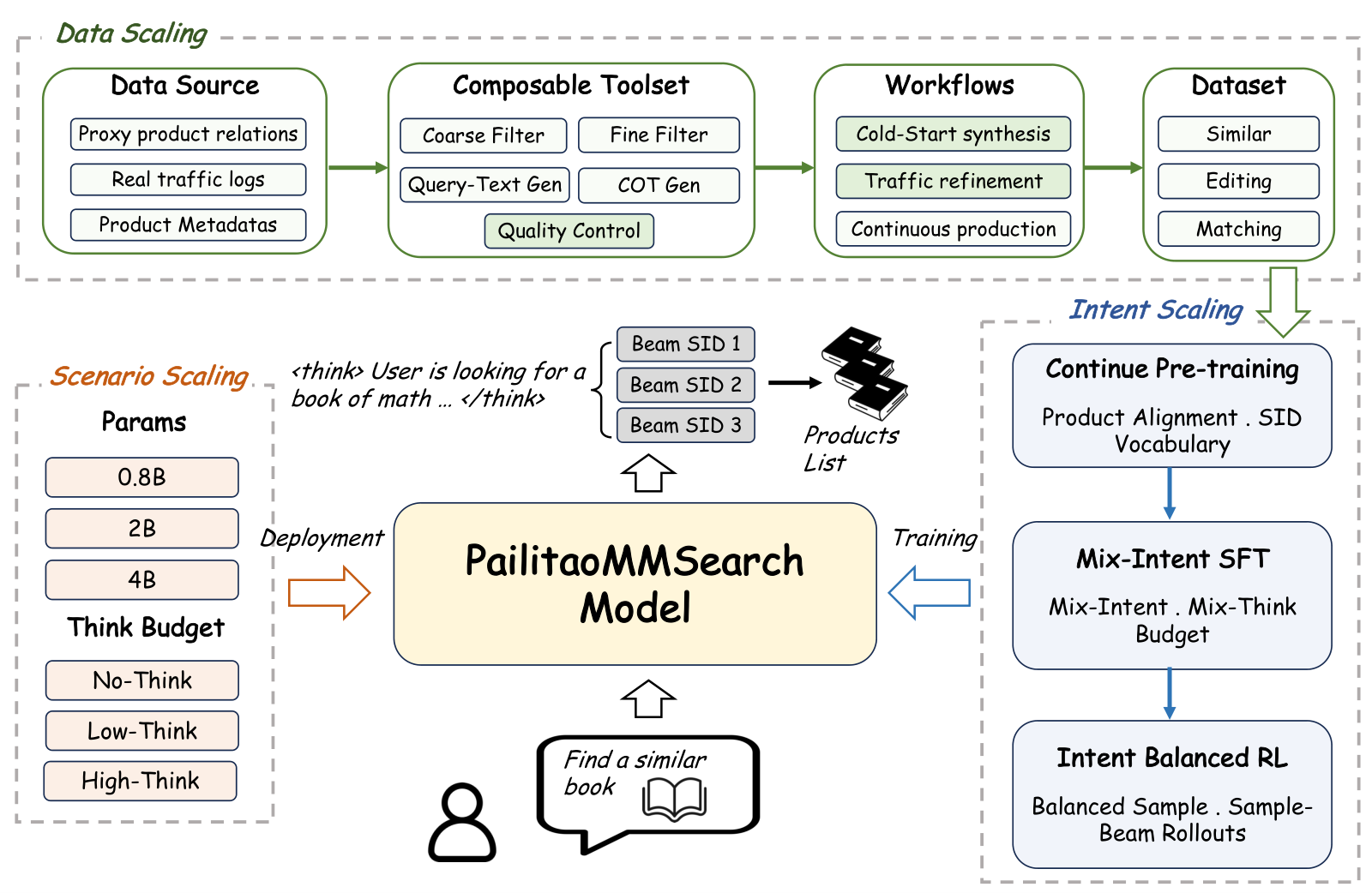 Generative · 2026-10-29PailitaoMMSearch2.0 Technical Report: Scaling Generative Retrieval to Unified End-to-End Multimodal SearchIn Taobao's Pailitao, a user may photograph a shirt and ask for shorts to match it, which calls for a complementary item rather than a duplicate. The usual pipeline classifies intent first and routes to separate retrieval channels, so one wrong step breaks everything after it. Alibaba's report lets a 2B vision-language model read the raw image and instruction and generate product Semantic IDs dir…
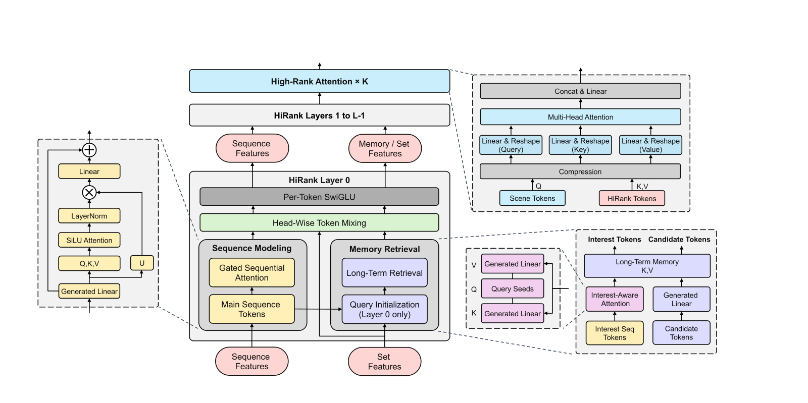 Personalization · 2026-10-28Unified Heterogeneous Feature Interaction via Effective-Rank Scaling for Recommender SystemsMost production ranking models squeeze the user's behavior sequence into one fixed vector before it reaches the feature-interaction module, so later interaction layers can no longer see which clicks or add-to-carts actually happened. Alibaba Taobao's HiRank keeps the behavior sequence alive through every layer of the backbone, and builds the retrieval query over long-term history from the user's…
 Generative · 2026-11-04Large Language Model as Universal Retriever in Industrial-Scale Recommender SystemIn this CIKM paper from Alibaba's Taobao and Tmall Group, one large language model handles click retrieval, per-scenario retrieval, long-tail retrieval, interest exploration and retrieval with a search query at the same time, and overall does better than the multi-task retrieval models common in industry. The user's history and the goal of this retrieval are written into one input. The LLM output…
 Generative · 2026-08-13UniScale: Synergistic Entire Space Data and Model Scaling for Search RankingDeep dive: UniScale: Synergistic Entire Space Data and Model Scaling for Search Ranking.
Discussion
Add experiment details, reproduction notes or a different take. Requires a GitHub sign-in.
Loading the discussion…