Contents · 8 sections
1What problem does it solve?2The overall picture3ES³: how the data grows fivefold4HHSFT: how the data is absorbed5Results6Limitations7How a ranking team might try it8VerdictSHARE

This paper is worth reading for teams that rank search or recommendation results and are thinking about making their model bigger. Its practical lesson: once parameters reach a certain size, the bottleneck is usually the training data, and the extra data only helps if the architecture is built to absorb it. The core idea of Taobao Search's UniScale in one sentence: turn unexposed candidates and user behaviour from other surfaces (recommendation feed, shop pages) into search training samples, which makes the training set five times larger, and then use a Transformer ranker that treats each feature type and each surface separately to absorb that data. Offline, the same expanded data lowers AUC by 0.43% (relative) on an architecture that does not separate surfaces, but raises it by 0.32% on the new one. In a 10-day online A/B test, purchases rose 1.70% and GMV 2.04%.
What problem does it solve?
Ranking models are usually trained only on search results that were actually shown: shown and clicked is a positive, shown and not clicked is a negative. The authors argue this causes three problems that get worse as the model grows.
The first is selection bias. Online, the ranker scores the whole candidate list, but during training it only ever sees the small top slice that was shown, never the clearly irrelevant candidates. The second is sparse labels. Purchases are credited to the last search click, so if a user saw an item in search and later bought it from the recommendation feed, that signal is lost. The third is a blind spot across surfaces. The many clicks and purchases on the recommendation feed and shop pages have no query and use a different feature format, so the search model cannot use them at all.
Here is an illustrative example used throughout. A user searches for "dress". The candidate list for this request has 100 items, 10 are shown, and she clicks one. The same day she buys, from the recommendation feed, a dress that had been shown in search but not clicked, and she also clicks a coat in the feed. Under the usual setup, only "one click, nine non-clicks" from all of this reaches the search model's training set.
The overall picture
The framework has two halves. The Entire-Space Sample System (ES³, the authors' name) expands the data, and HHSFT (Heterogeneous Hierarchical Sample Fusion Transformer, the authors' ranking architecture) absorbs it.
| Part | What it does | Training data size (relative to shown samples only) |
|---|---|---|
| Add unexposed samples | Randomly sample items that were not shown from each request's full candidate list | 3x samples, clicks unchanged |
| Hierarchical label attribution | Copy clicks and purchases from other surfaces onto search samples | 2x click positives |
| Cross-surface searchification | Give feed and shop clicks a query and turn them into search samples | 2x requests, 5x samples, 4x click positives |
| HHSFT feature interaction | Separate projections per feature type, then global interaction | No data change |
| HHSFT surface fusion | A shared expert plus one expert per surface, weighted by the current surface | No data change |
All data expansion happens offline, and only the search output is served, so online compute does not grow; the only extra cost is storage.
ES³: how the data grows fivefold
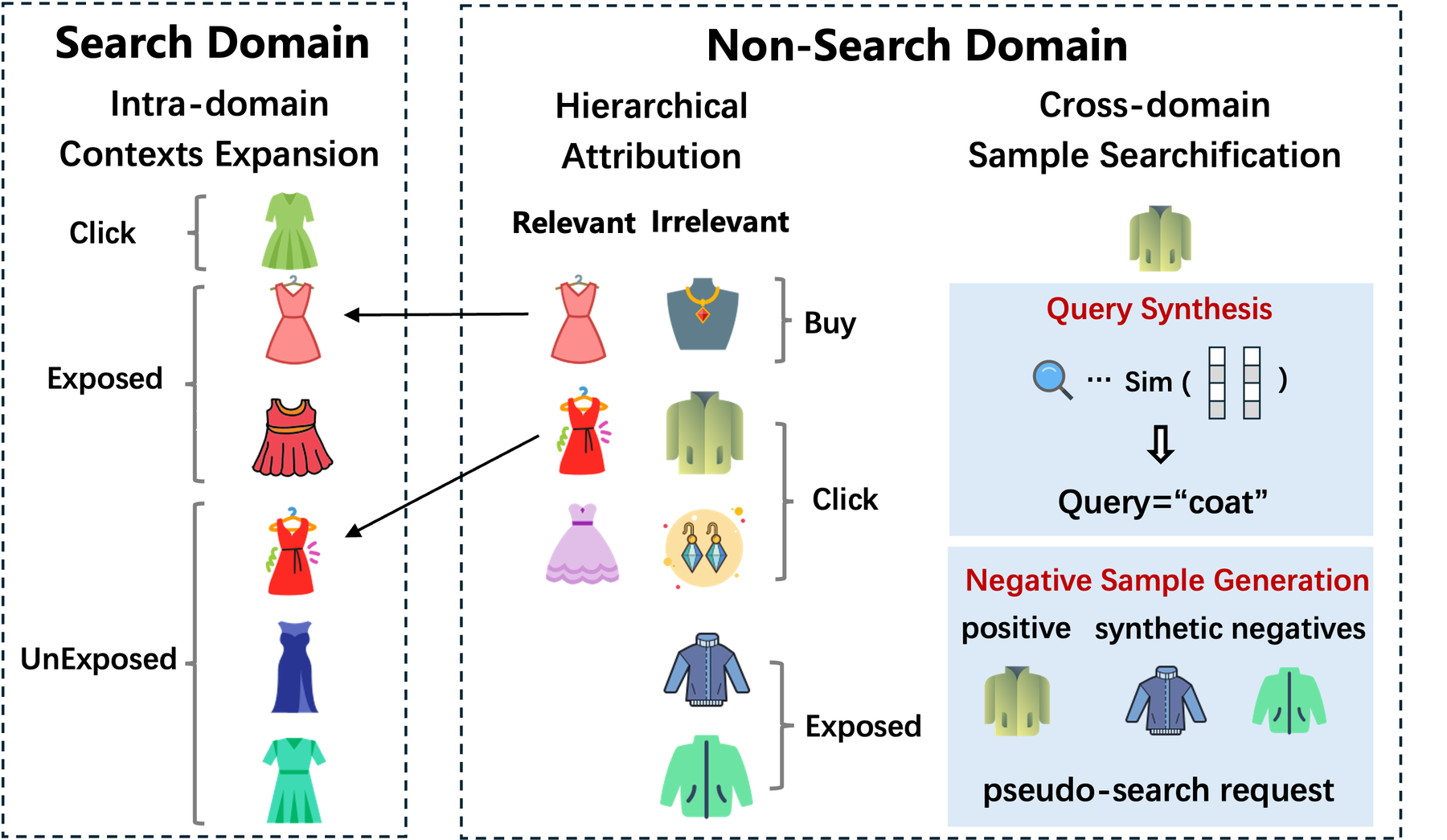
Adding unexposed samples brings the training distribution closer to the candidates the model scores online. In the example, some of the 90 unexposed items are sampled, and the request goes from 10 training rows to about 30.
But unexposed items cannot all be negatives. They were not shown because the old model did not rank them high, not because the user dislikes them, and training on that label every day pushes tail items further down in a self-reinforcing loop. So the authors relabel these samples with hierarchical attribution, which runs offline once a day and targets the same item the same user met in search. Clicks from other surfaces go first to a shown sample of that item, otherwise to an unexposed sample. Purchases from other surfaces go, in order of priority, to a search-click sample, then a shown-but-unclicked sample, then an unexposed sample. In the example, the dress bought from the feed had been shown in search but not clicked, so that row's purchase label flips from 0 to 1. The authors treat purchases such as same-day buys on item pages as an independent measurement of interest, because they happen outside the search exposure mechanism. This step doubles click positives.
Searchification handles the coat clicked in the feed. A feed request mixes unrelated items, so treating every unclicked item as a negative would add noise that has nothing to do with any query, and feed samples have no query field. The query is filled in by priority: first a query the user previously used to find this item, then a query that co-occurs with the item in search logs significantly more often than chance, and finally a nearest-neighbour search over query embeddings using the item title, with a minimum cosine similarity. Negatives are only items from the same feed request that are semantically similar to the clicked one but were not clicked. These samples then go through the search feature logging pipeline, so their format exactly matches real search samples. To cope with the larger data, each row now stores one request with all its candidates, which roughly halves storage and IO.
HHSFT: how the data is absorbed
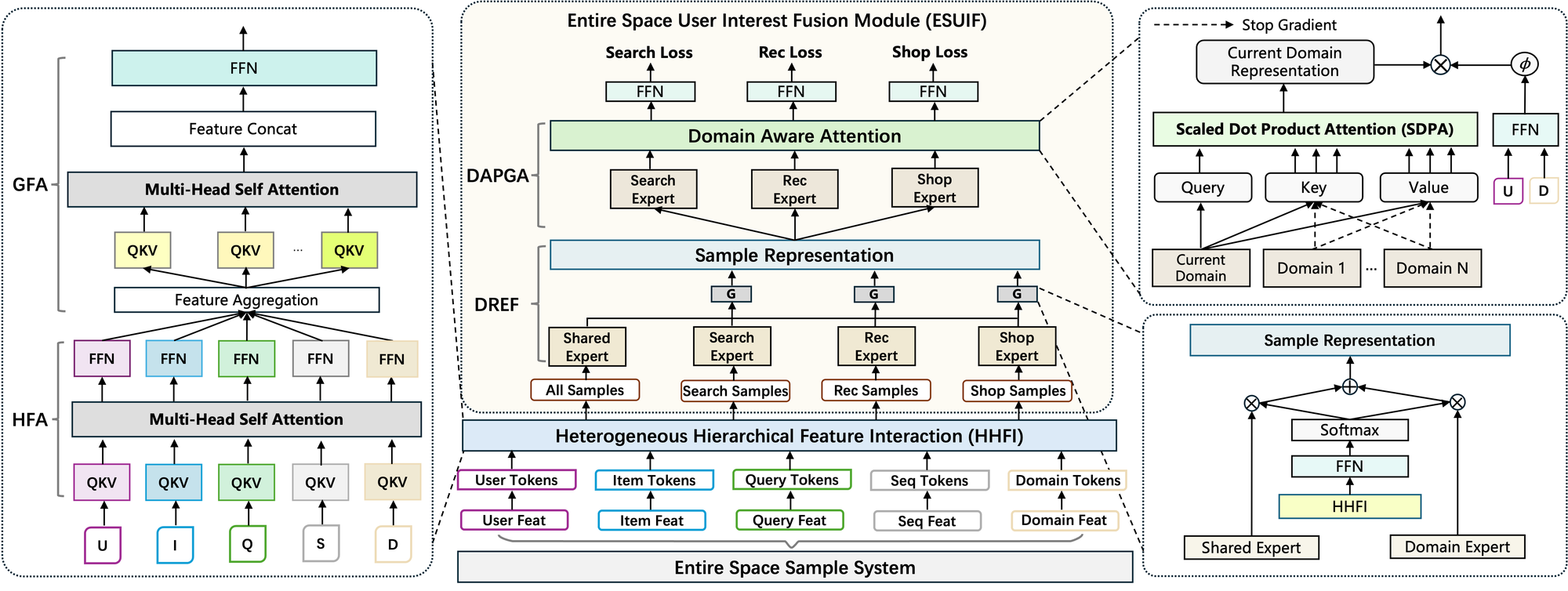
Heterogeneous feature attention (HFA) exists because a standard Transformer shares one set of query, key and value projections across tokens, while user IDs, prices and behaviour sequences come from very different spaces. HFA gives each feature block its own projections and FFN. Global feature attention (GFA) then concatenates all tokens and uses m projections to create new tokens that each see every feature; the base configuration uses m=8 tokens of 256 dimensions. In the ablation, swapping the MLP for a plain Transformer gives +0.17% AUC, adding HFA reaches +0.41%, and adding GFA reaches +0.80%. The authors call HFA plus GFA heterogeneous hierarchical feature interaction (HHFI).
Domain-routed expert fusion (DREF) has a shared expert that sees all samples and one expert per surface that only sees, and only learns from, its own surface. A gate weights the two per sample, for example 0.7 shared and 0.3 search. Domain-aware personalised gated attention (DAPGA) has its own set of surface experts. For a sample from a given surface, its own expert's output is the query, all experts' outputs are keys and values, and the other surfaces' paths are forward-only. Each surface has its own output head and cross-entropy loss, and only the search head is served. A sigmoid gate computed from user and surface features then scales each dimension of the result between 0 and 1.
Results
Main offline results, as relative AUC and GAUC gains over a DLRM-MLP baseline (Table 2 excerpt). The paper treats a 0.05% relative gain as a reliable improvement.
| Model | AUC | GAUC | Params (M) |
|---|---|---|---|
| DCNv2 | +0.08% | +0.01% | 24 |
| AutoInt | +0.26% | +0.14% | 150 |
| HiFormer | +0.54% | +0.49% | 170 |
| HHSFT, search data only | +0.82% | +0.62% | 300 |
| HHSFT + ES³ | +1.14% | +0.86% | 300 |
The key evidence is Table 4, relative to HHFI trained on search data only:
| Data | Architecture | AUC | GAUC | HR@5 |
|---|---|---|---|---|
| Search only | HHFI + DREF + DAPGA | +0.02% | +0.01% | +0.02% |
| ES³ | HHFI only | -0.43% | -0.24% | -4.76% |
| ES³ | HHFI + DREF + DAPGA | +0.32% | +0.26% | +0.44% |
Expanded data without the fusion layers is a net loss, with top-5 hit rate down 4.76%, and the fusion layers without new data do almost nothing. Only the combination pays off.
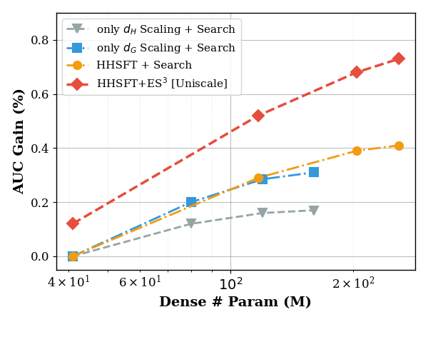
From about 40M to about 300M parameters, the search-only curve flattens after 100M while the ES³ curve keeps rising, and the gap widens from 0.12% to 0.32%. The authors call this a trend, not a scaling law, since the sweep covers only 7x. Online, 5% of traffic for 10 days against the production deep neural network (DNN) ranker gave +1.70% purchases and +2.04% GMV, and the engineering work cut GPU inference cost by more than half.
Limitations
All offline numbers are relative, with no absolute AUC, and each comes from a single training run. The online test changes architecture, data and serving optimisations at once, so it cannot say how much of the 1.70% comes from ES³; offline, the architecture alone accounts for most of the gain. Relabelled unexposed samples create a distribution gap that is left for the fusion layers to absorb, and HR@5 drops sharply without them. The scaling curve stops near 300M parameters.
How a ranking team might try it
First, change the architecture on existing search data: split features into blocks with separate projections and add a global attention layer, worth +0.80% AUC on its own. Second, add unexposed candidates and relabel them with purchases and clicks from other surfaces, which is cheap and gives about 3x samples and 2x positives. Third, only when non-search behaviour clearly outweighs search behaviour, add searchification together with the shared and per-surface experts, and check offline that the extra data hurts the old model but helps the new one. Watch top-5 hit rate as well as AUC, since negative transfer shows up there far more strongly.
Verdict
The most useful finding is that samples from other surfaces cannot simply be mixed into ranking training. They need an architecture that isolates gradients per surface, or more data makes results worse. The method borrows known parts, but the evidence for pairing data with architecture is clear, and the suggested rollout order is sensible for multi-surface e-commerce platforms.
How did this read for you?
Hoot made a note. Thanks for the feedback.

One tap, no sign-in; tap again to undo. Only anonymous counts are kept, never who you are.
Related papersMore from Paper Daily
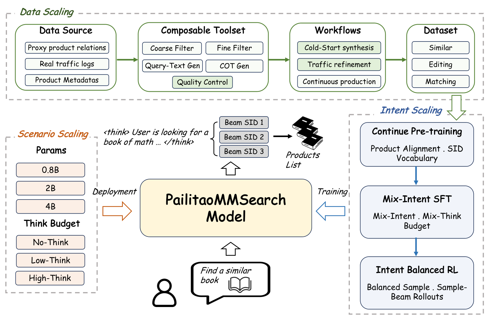 Generative · 2026-10-29PailitaoMMSearch2.0 Technical Report: Scaling Generative Retrieval to Unified End-to-End Multimodal SearchIn Taobao's Pailitao, a user may photograph a shirt and ask for shorts to match it, which calls for a complementary item rather than a duplicate. The usual pipeline classifies intent first and routes to separate retrieval channels, so one wrong step breaks everything after it. Alibaba's report lets a 2B vision-language model read the raw image and instruction and generate product Semantic IDs dir…
 Generative · 2026-11-02UGR: Unified Generative Ranking for Heterogeneous E-commerce RecommendationTaobao's generative ranking framework UGR has one generative model directly produce the screen the user finally sees. The roughly one thousand organic, ad and other-business candidates of a request go to the model together, and it generates the final list item by item, instead of each business ranking its own items and a blending stage stitching them together. That stitching step is the old probl…
 Generative · 2026-07-23TSGR: Taobao Search Generative RetrievalDeep dive: TSGR: Taobao Search Generative Retrieval.
 Personalization · 2026-10-28Unified Heterogeneous Feature Interaction via Effective-Rank Scaling for Recommender SystemsMost production ranking models squeeze the user's behavior sequence into one fixed vector before it reaches the feature-interaction module, so later interaction layers can no longer see which clicks or add-to-carts actually happened. Alibaba Taobao's HiRank keeps the behavior sequence alive through every layer of the backbone, and builds the retrieval query over long-term history from the user's…
 Personalization · 2026-08-28TransRetrieval: Scaling Up Transformer-Based Retrieval for Industrial RecommendationDeep dive: TransRetrieval: Scaling Up Transformer-Based Retrieval for Industrial Recommendation.
Discussion
Add experiment details, reproduction notes or a different take. Requires a GitHub sign-in.
Loading the discussion…