Contents · 7 sections
1What problem is it actually solving?2Core idea: compute exact distances only when needed3How the three components fit together4What the results show5Limitations as I see them6How a retrieval team could try it7Conclusion and assessmentSHARE

Teams building vector-search infrastructure, or running their own ANN index for RAG or recommendation, should read this. The paper proposes PAG (Projection-Augmented Graph), which adds a layer of random projection to a graph index. During search it first uses projections to estimate whether a neighbor could enter the candidate set, and computes the exact distance only for those estimated to make it; during graph construction it uses the same projection statistics to find extra incoming edges. The authors report that on 6 recent embedding datasets, single-thread search QPS is up to 5 times that of HNSW and indexing takes only 20% to 40% of HNSW's time. It stays ahead from 384 to 3072 dimensions and for K from 10 to 1000, and it supports online insertion. I think its value lies in fitting "fast search, fast indexing, insertable" into one framework with a clear idea; but it stores raw vectors as 16-bit floats while HNSW and Vamana store 32-bit ones, which mixes into the memory and speed comparisons, and some of the most striking high-dimensional conclusions are affected by a baseline implementation defect.
What problem is it actually solving?
The authors' starting point: older ANN evaluations (such as ANN-Benchmarks) mostly use hand-crafted image features like SIFT and GIST from over twenty years ago, and only compare QPS-recall curves at K=10; today's applications ask for more. The paper lists six demands: fast search (D1), fast indexing (D2), moderate and adjustable memory (D3), handling embeddings with thousands of dimensions (D4), stability for K from 10 to the thousands (D5), and online insertion (D6).
Each existing family has a weak spot. Graph indexes (HNSW, Vamana) search fast but build slowly, computing exact distances at every step. Quantization methods (IVFPQ, ScaNN, RaBitQ+) build fast and save memory, but their QPS-recall trails graphs. Quantized graphs (SymQG) search very fast, but are sensitive to the data distribution and do poorly on high dimensions, large K and insertion. Projection-plus-graph methods, such as the authors' earlier KS2 (a random-projection routing test), cut exact distance computations during search, at the cost of slower building, more memory and harder insertion.
A running illustrative scenario: a team has a knowledge base of 1 million documents encoded with the 3072-dimensional text-embedding-3-large, adds several thousand documents a day, and retrieves the top 100 online before reranking. This scenario hits high dimensionality, large K and continuous insertion at once, exactly the situation PAG aims to cover.
Core idea: compute exact distances only when needed
Search in a graph index is a greedy walk: from the current node , check how far each out-neighbor is from the query , put the close ones into the working set , then pick the next node from the working set and keep going. The main cost is computing , each time an operation on a 3072-dimensional vector. Yet most neighbors turn out, after the computation, to be farther than the farthest point in and cannot enter the working set, so that computation is wasted.
PAG first runs a cheap test that answers only "could enter the working set". The authors borrow a result from KS2. With vector norms stored in advance, " is closer than the current farthest point " is equivalent to the cosine of the angle between and exceeding a threshold . This threshold can be computed from three distances: was already computed before the walk reached , is at hand in the working set, and the edge length can, in the paper's words, be precomputed; the paper's account of where it is read from at search time stops there.
The remaining question is how to estimate this cosine without a high-dimensional inner product. PAG first applies one fixed random orthogonal transform to all data, then cuts the dimensions into blocks of dimensions each. Each block gets a codebook of randomly rotated unit vectors, all scaled by . Concatenating one vector from each block's codebook gives a projection vector of length exactly 1. During indexing, for each edge , PAG picks in each block the codebook vector with the smallest angle to that block of (the index takes only 4 bits) and concatenates them into the projection vector . It also stores the cosine between and , plus 's projection values on those codebook vectors. The transform matrix is fixed, and each incoming query is first multiplied by the same matrix before anything else, so the table lookups and the statistics stored on edges live in the same coordinate system. When a query starts, 's projections on all codebook vectors are computed once and stored as a projection table. After that, checking any edge only means looking up the table with that edge's stored indices, subtracting 's projection values and summing, which gives the projection of on ; dividing by the known gives . This step is just lookups and additions, never touching a -dimensional vector. The paper's Theorem 3.1 proves that when and each block's dimension are large enough, is approximately Gaussian with mean , where is the angle to be estimated. So the test function is:
Only a positive value triggers the exact distance. The paper calls this test PRT (Probabilistic Routing Test). In complexity, HNSW search is and PAG is , where is the number of visited nodes, the maximum out-degree, and the fraction of neighbors passing the test, which the authors say is generally below 0.2 in practice. is much smaller than ; the appendix recommends a value between 8 and , and the experiments use 16 to 128.
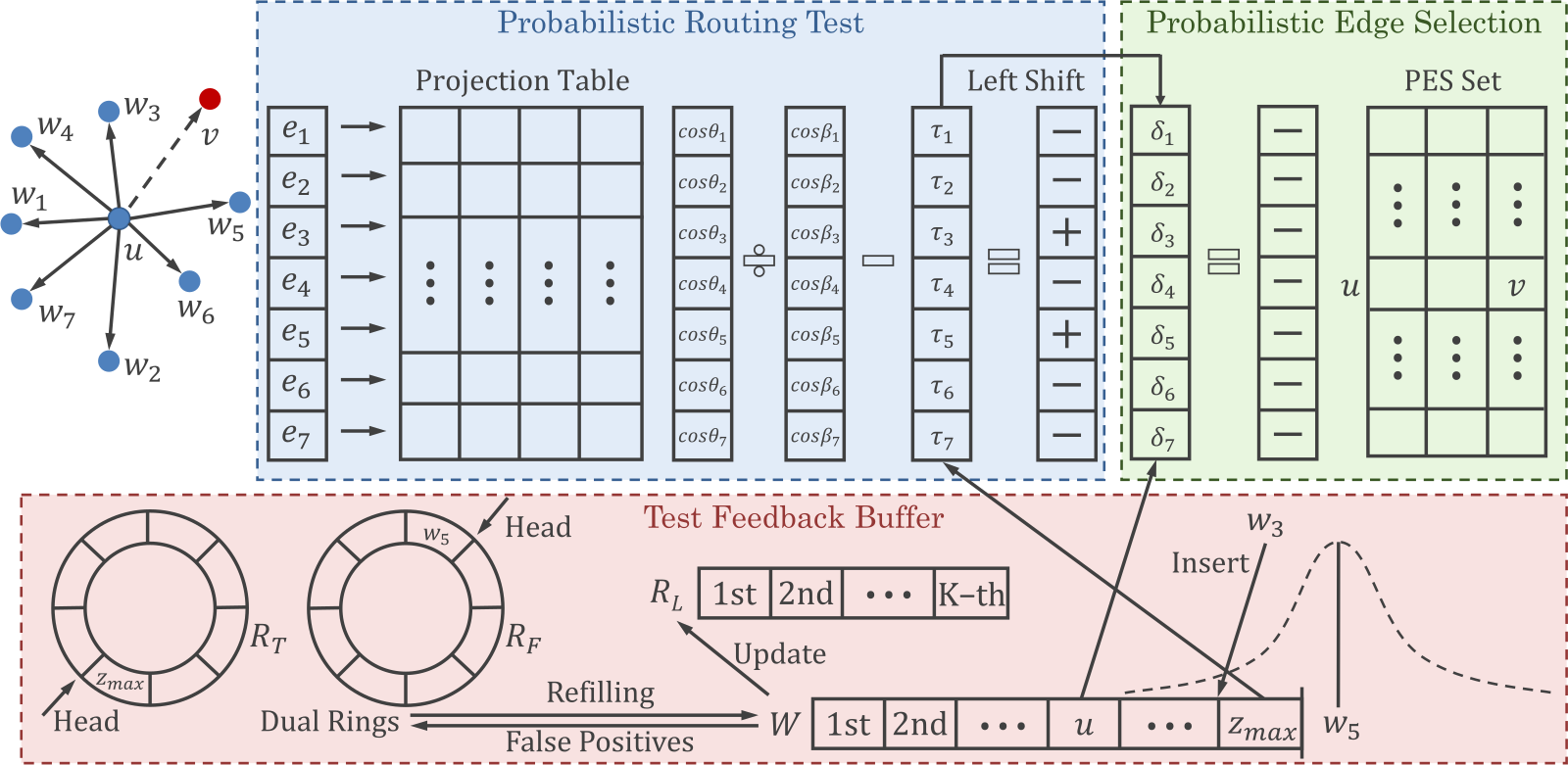
In the scenario: the query reaches node , which has 7 neighbors. Plain HNSW computes 7 distances in 3072 dimensions; PAG first runs 7 projection tests, each involving only lookups over blocks and a few multiply-adds, and if, say, only 2 pass, it computes just 2 exact distances.
How the three components fit together
The first component is TFB (Test Feedback Buffer). PRT is a probabilistic test and has false positives: neighbors that pass the test but, once their exact distance is computed, cannot enter the working set. Earlier methods such as KS2 simply discard them, wasting the exact distances already computed. Why handle them specially? Because the Gaussian distribution from Theorem 3.1 implies these false positives are usually only slightly beyond the threshold, so they are likely to be useful in later rounds. TFB splits search into rounds: each round runs best-first search on a small working set , points pushed out of go into ring buffer , and false positives go into . Once every point in has been visited, the round ends: those points move to the result list, is cleared, and the two rings are merged and sorted by distance, filling first and returning the rest to . The points in the new round's are farther than the previous round's, so the farthest point is farther too and the test threshold loosens; the previous round's false positives can now mostly enter , and their exact distances, already computed, need not be recomputed. During search, 's size is the larger of 10 and K. The search budget is set by the parameter efS, which the paper's text calls the maximum number of visited nodes; what the algorithm actually does is divide efS by 's size (rounded up) to get the maximum number of rounds, stopping early if empties. Because keeps taking in new points within a round, the cumulative number of visits can exceed efS, so efS is best read as an approximate per-round budget. The threshold is set by the farthest point in rather than the whole result queue, so is small, the threshold is tight and elements move quickly.
The second component is PES (Probabilistic Edge Selection). HNSW and Vamana decide edges with RobustPrune. Its rule: for a candidate node , suppose some out-neighbor of is no farther from than is, and no farther from than is. Then counts as reachable from via , so the direct edge is redundant and not kept. The edge is kept only if no such "witness" exists. When finding incoming edges for a new node , candidates are limited to 's out-neighbors. Prior work has pointed out that this leaves some nodes with very small in-degree, nearly unreachable during search, which is one reason HNSW performs poorly on some real data. Simply enlarging the candidate set is expensive, since RobustPrune's worst-case cost per candidate is . During indexing, the new node being inserted is the query of that search: builds its own projection table on arrival, so the obtained at each visited node estimates the angle between and . PES reuses these ready-made estimates and only swaps in another threshold : a cosine above it means is closer to than is. PES computes , that is, it checks whether any of 's out-neighbors has an estimate above the threshold: a positive result means a witness may exist; a negative result means none was found. When it is negative, the edge is probably not redundant, so it is recorded in the candidate buffer , up to per node, to be verified later in batch by RobustPrune. The key point is that PES can check every node visited during the construction search, not just 's out-neighbors. can be computed from quantities PRT already has, so each neighbor costs only extra work.
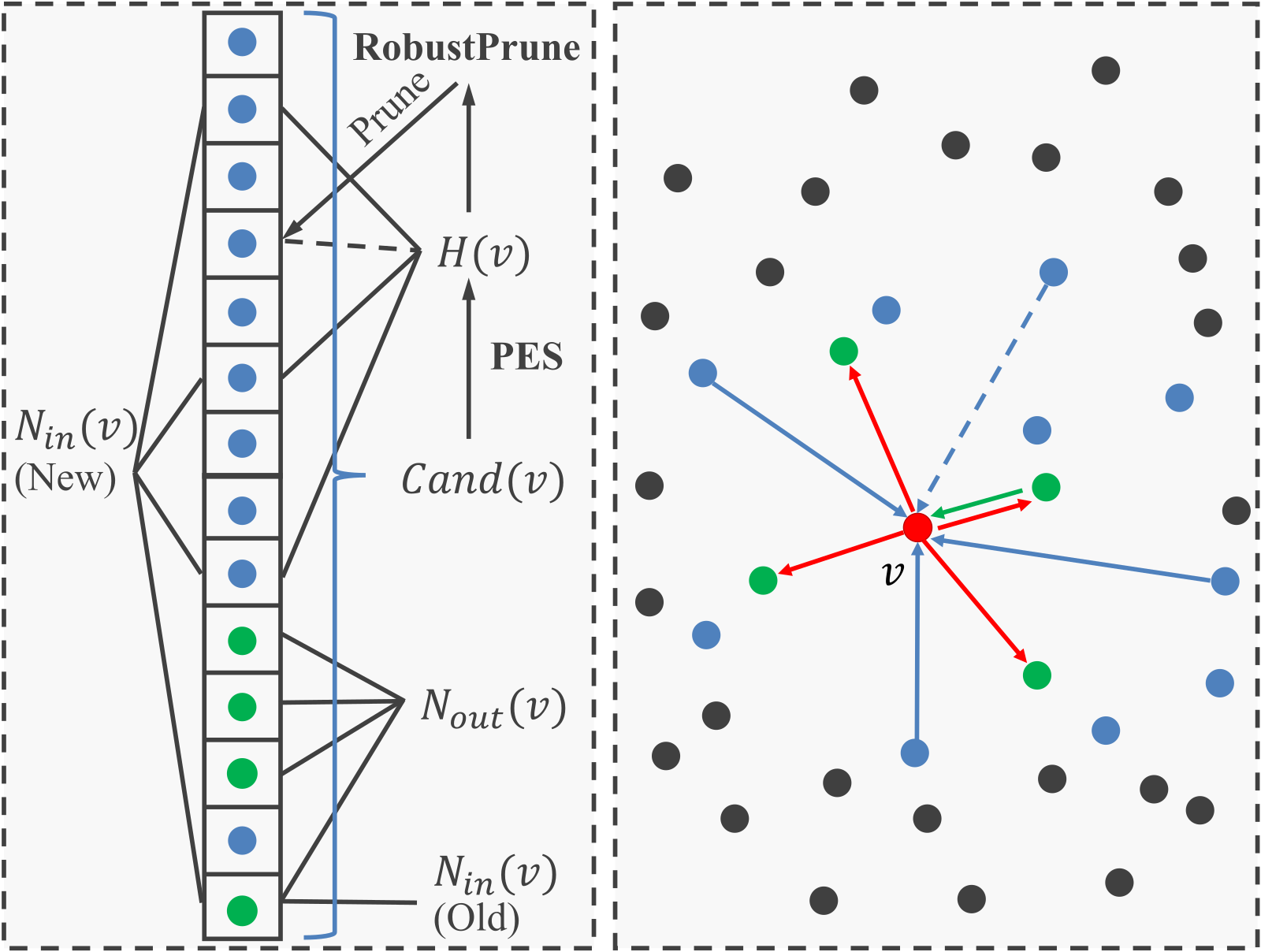
The three components chain together during indexing as follows. PAG inserts vectors one by one. Step one uses search with PRT-TFB to find candidates, then RobustPrune to set outgoing and incoming edges; step two uses PRT-PES to pick extra candidate incoming edges from all visited nodes and stores them in ; step three applies RobustPrune to those candidates to set the final incoming edges. Because building the graph is itself "search, then insert", speeding up queries also speeds up indexing. Online insertion follows the same flow, except that PES candidates are verified together only after enough new nodes have been inserted to form a batch, and until then these candidate incoming edges are not yet in the graph; verified edges only fill out-edge slots that are still free, and existing edges are left alone. The verification cost amortizes to per inserted node. The several thousand documents added each day in the scenario are inserted one by one this way, without rebuilding the index.
What the results show
The main experiments use 8 datasets: 6 new ones produced by recent embedding models and 2 widely used older ones:
| Dataset | Size | Dim. | Type | Embedding model |
|---|---|---|---|---|
| DBpedia1536 | 999,000 | 1,536 | Text | text-embedding-3-large |
| DBpedia3072 | 999,000 | 3,072 | Text | text-embedding-3-large |
| WoltFood | 1,719,611 | 512 | Image | clip-ViT-B-32 |
| DataCompDr | 12,779,520 | 1,536 | Text-to-image, out-of-distribution queries | coca_ViT-L-14 |
| AmazonBooks | 15,928,208 | 384 | Text | all-MiniLM-L12-v2 |
| MajorTOM | 56,506,400 | 1,024 | Image | DINOv2 |
Baselines are HNSW, Vamana, SymQG, ScaNN, IVFPQFS and RaBitQ+. PAG comes in two parameter settings: PAG-Base for search speed and PAG-Lite for fast indexing and small memory. Search is single-threaded and indexing uses 112 threads, on a Xeon server with AVX-512. The default is K=100.
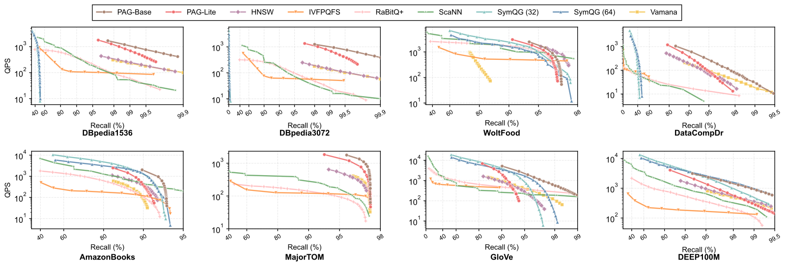
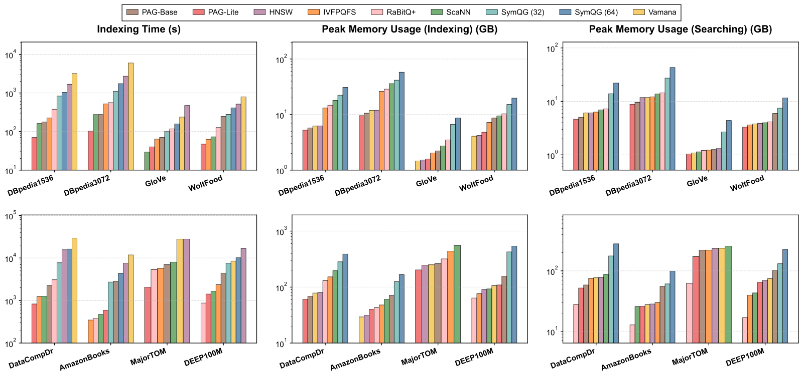
On search speed, PAG-Base is best on all 6 new datasets except the high-recall range on WoltFood, up to 5 times faster than HNSW; on the older data it is best on GloVe and second only to SymQG on DEEP100M. PAG-Lite ranks second on DBpedia1536, DBpedia3072 and MajorTOM. On indexing time, PAG-Base needs only 20% to 40% of HNSW's time and is faster than SymQG in most cases; PAG-Lite is on par with quantization methods and fastest on high-dimensional data. On memory, PAG-Lite has the smallest indexing and search memory on 4 of the 8 datasets; PAG-Base uses more than HNSW on low-dimensional data, with a negligible difference at high dimensions.
As K varies: at K=10, PAG-Base is on par with SymQG and better in the high-recall range above 95% on every dataset except DEEP100M; at K=1000, PAG-Base is still best while SymQG degrades clearly, and the gap widens as K goes from 200 to 800. In the online-insertion experiment, 10,000 vectors are randomly drawn from the corpus for insertion and another 10,000 for queries, split into 20 interleaved batches. PAG-Base is faster than HNSW at both insertion and search, and its insertion is even faster than HNSW's search; compared with HNSW's insertion, it is up to 5 times faster. This shows applying the projection test to both indexing and search really does free a graph index from choosing between fast building and fast search.
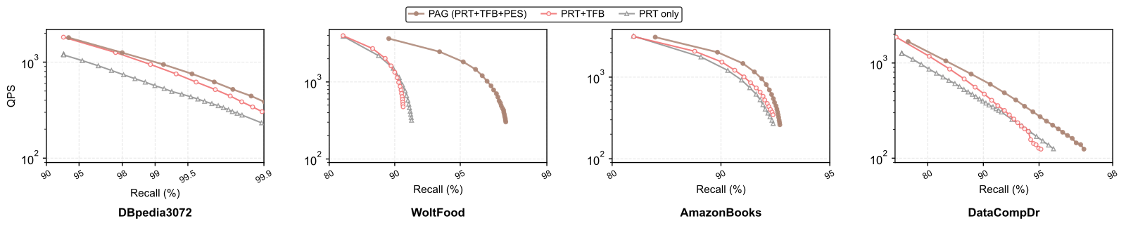
The ablation shows TFB reduces indexing time and improves search on all 4 datasets; PES improves search further, most visibly on WoltFood, where recall without PES stalls just above 90% and adding PES shifts the whole curve right, with almost no change in indexing time. PES pays off most on hard data, which matches what it was designed for: adding incoming edges so that nodes with very small in-degree can still be reached during search.
Limitations as I see them
First, storage precision differs. The appendix says PAG stores raw vectors as 16-bit floats while HNSW and Vamana store 32-bit, so PAG's data payload uses less memory. Exact distance computations also read half as much data, which may help both search and indexing speed. The paper lacks a control with HNSW also using 16-bit storage, so the existing results cannot separate how much of the memory and speed advantage comes from this.
Second, a baseline has an implementation problem, and parameters are tuned per dataset. SymQG has very low recall on the 1536- and 3072-dimensional data; the authors explain in a footnote that its source code uses an unsigned 16-bit integer type for parallel computation, which overflows at high dimensions. That means the conclusion "PAG far outperforms quantized graphs at high dimensions" partly comes from comparing against a broken baseline. On GIST and SIFT10M (which the authors call sparse and well suited to quantization), SymQG still has higher QPS at K of 10 or 100, and on DEEP100M PAG-Base only comes second. PAG-Base's parameters are set per dataset. On the six modern datasets its efC (the maximum number of nodes visited per insertion during indexing; larger means better graph quality and slower building) ranges from 1000 to 2000, and M is 128 on WoltFood, while HNSW uses efC=1024 (512 on MajorTOM) and M=32. Appendix G.5 adds a comparison at equal efC, where PAG-Base is still better, but that comparison only aligns efC; the difference in M remains.
Third, the conclusions rest mainly on curves, and the evaluation scope is limited. "Up to 5 times" is the largest gap along the curves, with no table of values at fixed recall; search is tested single-threaded only, with no multi-thread throughput and no comparison with disk indexes such as DiskANN. The online-insertion experiment inserts only 10,000 vectors, with no deletions and no test of whether graph quality degrades after long periods of insertion. Theorem 3.1 is asymptotic; for finite codebook size and block count , there is only a weaker guarantee from the KS2 paper: when the cosine of the angle is truly at least the threshold , the test passes with probability at least 0.5.
How a retrieval team could try it
- On your own embeddings and real queries, compare single- and multi-thread QPS of PAG-Base and HNSW at two recall points, 95% and 99%, and add an HNSW run with 16-bit storage as a control to separate out the effect of storage precision.
- If your K is in the hundreds or more (recommendation retrieval, image search), focus on the large-K curves, where PAG's advantage in the paper is most stable.
- For workloads with continuous writes, simulate a week of insertions and measure recall periodically to see whether graph quality holds; also record daily insertion time and compare it with the time to rebuild HNSW.
- Start from the appendix's suggested parameters: efC of at least 800 for fast search, efC of at most 200 for fast indexing and small memory, M of 32 or 64, between 8 and , then tune to your memory budget.
Conclusion and assessment
The key takeaway: most exact distance computations in a graph index are wasted; screening first with a cheap probabilistic test, whose statistics can also improve graph construction along the way, lets search, indexing and insertion all get faster together.
| Dimension | Assessment |
|---|---|
| Problem importance | High. High-dimensional embeddings, large K and continuous insertion are the norm for RAG and recommendation retrieval |
| Method novelty | Medium. PRT follows the ideas of KS2 and earlier work; the novelty is TFB reusing false positives, PES edge selection, and applying projection to graph construction |
| Experimental evidence | Medium. New datasets, full coverage of the demands, ablations and an equal-parameter comparison; but storage precision differs, SymQG has an implementation defect, and results are curves only |
| Engineering cost | Medium. Code is open source; the implementation is designed around AVX-512, has one more parameter than HNSW, and must be tuned per dataset |
| Worth trying? | Worth benchmarking on your own data, especially for high-dimensional, large-K, continuous-insertion workloads; remember to add a 16-bit HNSW control |
How did this read for you?
Hoot made a note. Thanks for the feedback.

One tap, no sign-in; tap again to undo. Only anonymous counts are kept, never who you are.
Related papersMore from Paper Daily
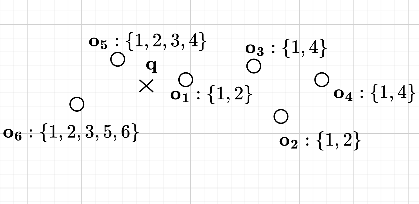 Infra · 2026-11-13Dynamic Graph Indexing for Label-Filtered Approximate Nearest Neighbor SearchVector retrieval often comes with a filter, such as finding nearest neighbors only within a few tags or categories. The hard part is that once a graph index like HNSW is filtered by label, many edges get cut, qualifying points can no longer reach each other, and the search gets stuck locally. DYLAN arranges objects by their label sets in a prefix trie, builds shared graph indices on only some tri…
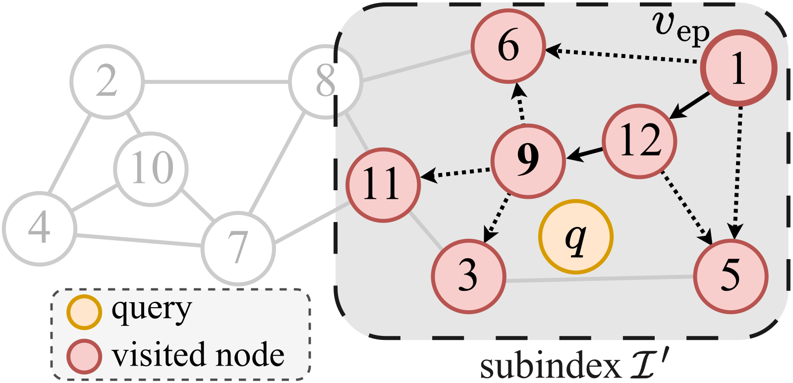 Infra · 2026-11-16Authenticated Approximate Nearest Neighbor Search in Outsourced Vector DatabasesOnce a vector database is outsourced to a third-party cloud, the provider may skip neighbors to save compute or even tamper with results, so the client needs a way to verify that a nearest-neighbor search is genuine. Existing methods have the cloud send back the traversal path on the graph index along with every raw vector visited on the way, and the client recomputes the distances itself. Embedd…
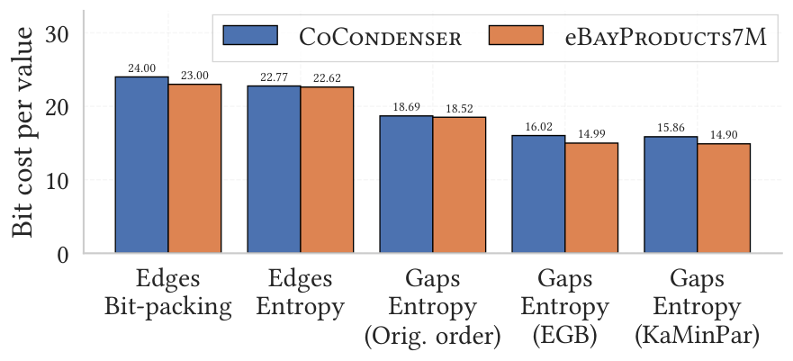 Infra · 2026-10-29Lossless Compression of Proximity Graph Indexes for Efficient Approximate Nearest Neighbors SearchIn HNSW graph indexes for vector search, the vectors are often already quantized, so the edges in the adjacency lists become the main memory cost. Edges are decoded on the fly while each query walks the graph, so compression cannot slow queries down. This work from eBay and the University of Pisa renumbers nodes offline so that neighbors get nearby IDs, then decodes with the SIMD-friendly integer…
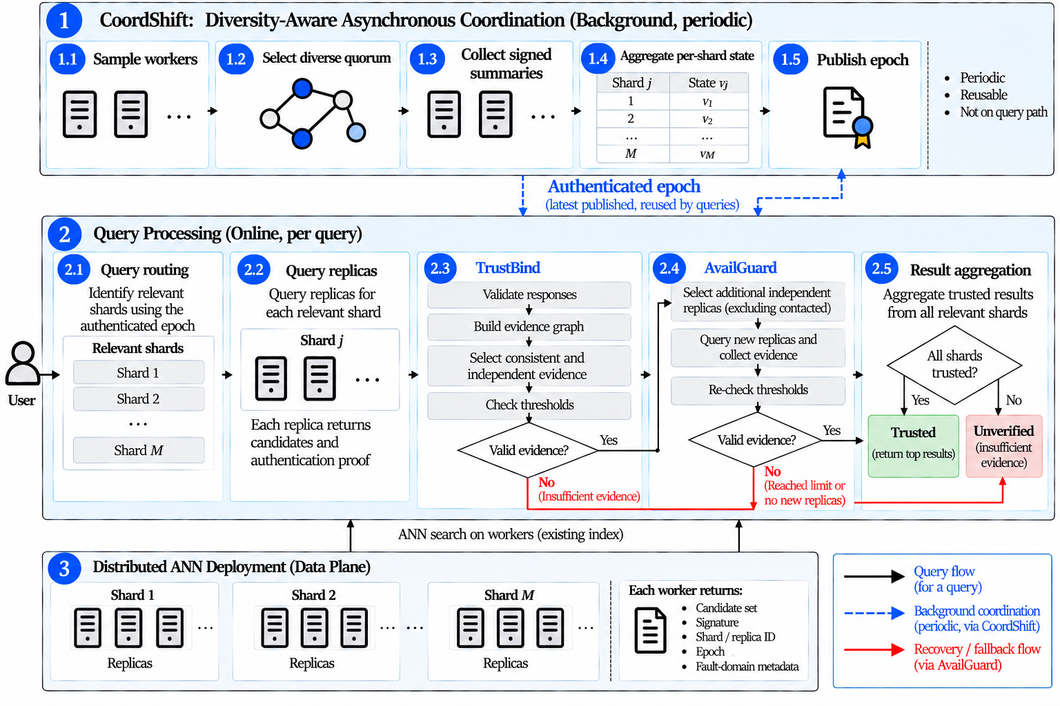 Infra · 2026-10-28Failure-Resilient and Verifiable Distributed Approximate Nearest-Neighbor RetrievalReplicas in a distributed vector database keep results available but do not make them trustworthy. A compromised replica can return validly signed but tampered nearest neighbors. TrustANN adds middleware above the router. For each shard it greedily picks a set of replica replies that meets a set minimum size, scores high on pairwise similarity (candidate overlap plus rank agreement), and spans a…
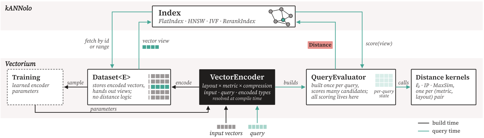 Infra · 2026-11-05Modular and Efficient Approximate Nearest Neighbors Search with Vectorium and kANNoloIn vector search, switching to another embedding form or quantizer often means switching libraries. Existing ANN libraries either support one combination or write separate code for each, and no ANN library covers dense, sparse and multi-vector embeddings behind one interface. The authors release two open-source Rust libraries to fix this: Vectorium stores vectors, computes distances and quantizes…
 Retrieval · 2026-11-11Lightfoot: Graph Retrieval-Augmented Generation with Exact, Model-Free Document DeletionGraphRAG in production has two costs that papers rarely count: what it takes to build the graph, and how painful it is to delete a document. When a contract expires or a user asks for erasure, a document and everything derived from it must go, yet entity summaries that blend several documents are hard to take apart. Lightfoot requires every record in the graph to be computed only from single-pass…
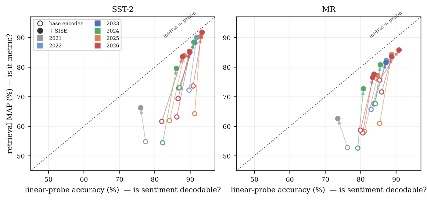 Retrieval · 2026-10-26Semantically Rich, Metrically Affect-Blind: A Geometric Blind Spot in Modern Text EmbeddersSearch a vector index for what users dislike about a product, and the reviews you get back are usually on topic but a mix of praise and complaints. This paper measures why. Across 11 text embedding models, sentiment is present in the vectors and a simple linear classifier can read it, yet the cosine similarity that retrieval actually uses barely registers it. A small projection head on the frozen…
Discussion
Add experiment details, reproduction notes or a different take. Requires a GitHub sign-in.
Loading the discussion…