Contents · 8 sections
1How much has to be sent to verify one search2Verifying distances without sending vectors3Growing the Merkle tree along the search path4Walking through it: 7 visited nodes, what goes into the VO5Adding quantization: pruned candidates skip exact authentication6Results7What this means for people running vector search services8LimitationsSHARE

You outsource vector search to the cloud: how do you know it didn't cut corners? VIDA lets the client verify without receiving the raw vectors of the nodes the search passed throughYour company hands 100 million text embeddings and an HNSW index to a cloud provider. For every query it returns the 100 nearest neighbors. The problem is that you cannot tell whether it actually finished the search. It could take a few fewer steps, stop early, return a "close enough" answer and save itself the compute.
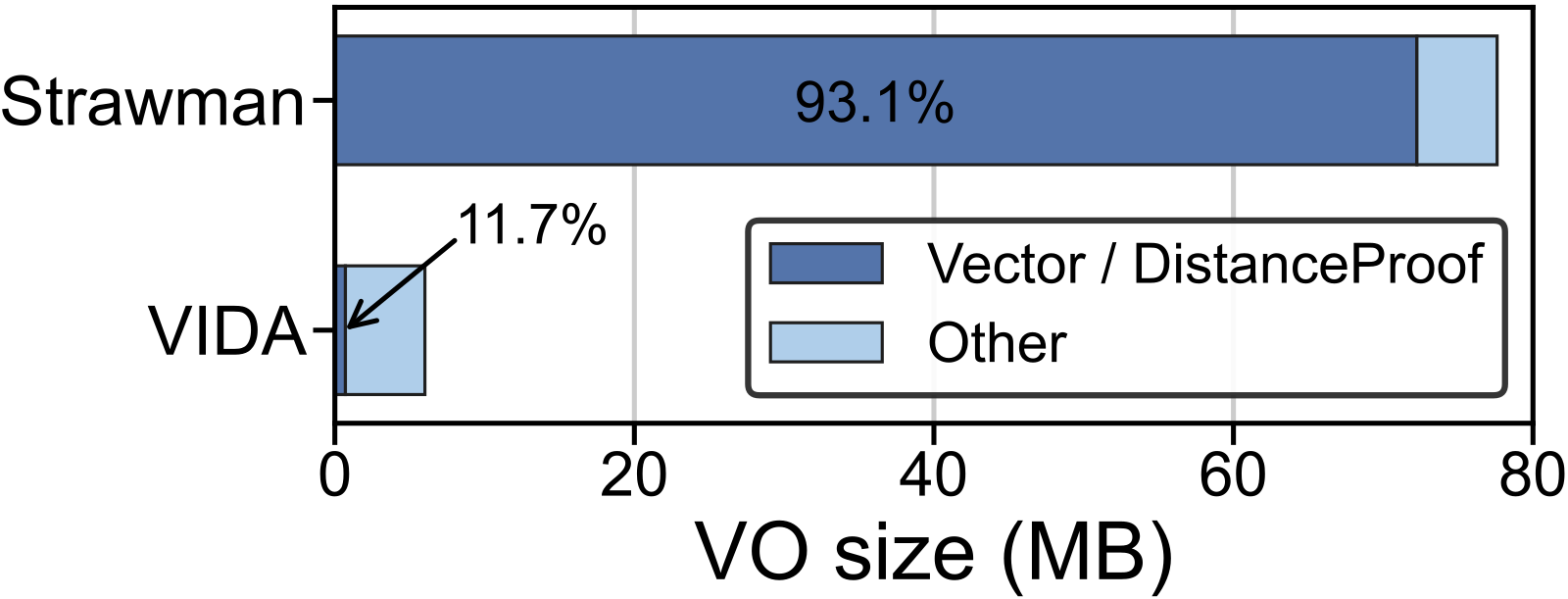
The existing way to check is to have the cloud attach a proof to the results, called a verification object (VO). The client replays the search locally with it and accepts the results only if they match. The catch is that this proof contains the raw vector of every node visited during the search. On the 3072-dimensional OpenAI3072 dataset, a single query's VO is 77.61 MB, and raw vectors make up 93.1% of it.
This paper, from Hong Kong Baptist University, studies how to verify approximate nearest neighbor (ANN) search on graph indexes without sending the client the raw vectors of the nodes the search passes through. The existing approaches, Strawman and ANNProof, authenticate graph nodes with a Merkle hash tree and then send all visited raw vectors to the client so it can recompute distances; the Merkle tree is built by node ID and has nothing to do with the search path. The paper's scheme, VIDA (verifiable inner-product-based distance authentication), changes three things. For the nodes the search passes through, it sends only each vector's commitment and norm, and only the final results' raw vectors still go to the client for checking; it authenticates distances with an Inner Product Argument (IPA, a cryptographic protocol that proves "the inner product of two vectors equals some value") and merges all nodes' proofs into one. It builds the Merkle tree along the graph structure (MeST) and issues proofs only for nodes that were actually expanded. And when combined with quantization, candidates pruned by a lower bound no longer need exact authentication. At the highest recall target on OpenAI3072, VIDA*'s end-to-end latency is 6.6 times faster than ANNProof and its transmission time is 99.2% lower.
What the client has to verify is distances, and a distance needs only two norms and one inner product, so the raw vectors of the nodes along the way can be replaced by fixed-size commitments plus one merged proof; the cost is that the data owner's index build takes about 5.5 times as long as before.
How much has to be sent to verify one search
First, who does what. The data owner builds the graph index, builds an authenticated data structure (ADS, most commonly a Merkle hash tree) on top of it, signs the tree's root, and hands everything to the cloud. The cloud answers queries and produces a VO for each result. The client verifies with the VO. The cloud is untrusted; the data owner and the client are honest.
What is verified here is not "are these the true top 100 neighbors". ANN is approximate by design, and exact verification is too expensive. What is verified is execution integrity: the results the cloud returns must be exactly what faithfully running the same deterministic search algorithm would produce.
Search on a graph index goes like this. Starting from an entry node, it keeps a priority queue sorted by distance to the query. Each time it takes out the closest candidate, computes distances for all of that node's neighbors and puts them in the queue. It stops when the candidate it takes out is farther than all k results already found, and those k are the result.
Strawman has the cloud package every node whose distance was computed during the search: node ID, adjacency list and raw vector, plus Merkle proofs for these nodes and the data owner's signature. The client first recomputes the tree root from the Merkle proofs and checks the signature, confirming the nodes were not altered. It then assembles these nodes into a subgraph and replays the search on it. The check passes only if the replay matches the cloud's result and never reaches a node outside the subgraph.
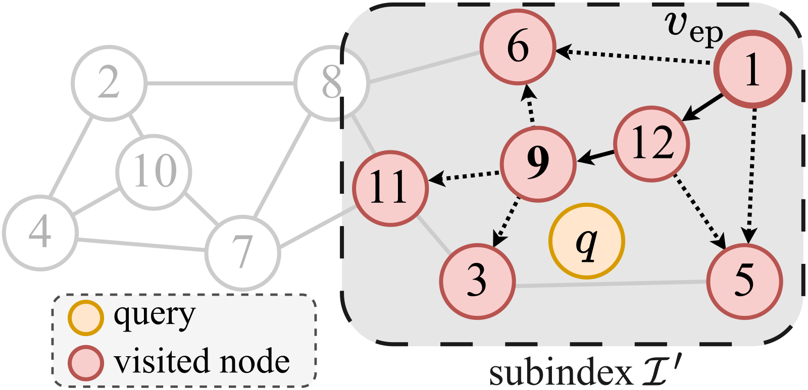
There are two problems. First, raw vectors are large. The higher the recall requirement, the more nodes the search visits and the more vectors must be sent. Second, the Merkle tree is ordered by node ID, unrelated to the search path. In the paper's example, v1, v9 and v12, which the search visits together, share only the root in the tree, while consecutively numbered v1, v2 and v3 share deep ancestors, so the proofs cannot be compressed.
Verifying distances without sending vectors
So what does the client actually need from a vector? The authors observe that Euclidean distance, cosine similarity and inner product all depend on just three things: the norm of the query vector, the norm of the data vector, and their inner product. For Euclidean distance, squared distance = squared data norm + squared query norm − 2 × inner product.
The query vector belongs to the client, so it computes that norm itself. The data vector's norm is computed by the data owner when building the ADS and placed under the signature. All that is left to prove is the inner product.
VIDA uses Pedersen vector commitments. You can think of a commitment as a "fingerprint" of a vector: it has fixed size regardless of dimension, and the cloud cannot later claim it belongs to a different vector. The data owner computes a commitment for each vector and puts it, together with the norm, into a leaf of the Merkle tree. At query time, the cloud provides the inner product and an IPA proof for each visited node, and the client verifies that the inner product is genuine using the commitment and its own query vector.
One IPA proof per node is still too much, since a high-recall search often visits over a thousand nodes. All these inner products have one thing in common: the other side is always the same query vector. VIDA therefore merges them with a random linear combination: it derives a random number r from the public commitments and inner products, multiplies the i-th vector by r to the power i, adds them up, and runs a single IPA between this combined vector and the query vector. The client combines the commitments and inner products with the same coefficients and verifies just that one proof. The paper proves this merging is secure.
Growing the Merkle tree along the search path
The remaining cost is in the Merkle proofs. MeST builds a spanning tree on the graph rooted at the entry node and then builds the Merkle tree along that spanning tree.
The tree is built in layers by hop count: nodes one hop from the entry go in the first layer, two hops in the second, and so on. When a node can be reached from several nodes in the layer above, the one closest in vector distance becomes its parent. Why not use an ordinary minimum spanning tree? Looking only at hops ignores that greedy search prefers close neighbors; looking only at distance can make the tree very deep and the proof paths long.
What each node stores in the tree changes too. Node v's record holds the IDs, commitments and norms of all its neighbors, not its own vector. With v's record, the client can authenticate the distance from each of v's neighbors to the query. A neighbor's own record is sent only when that neighbor is actually expanded.
This splits the nodes into two sets. Many nodes have their distances computed, and all their inner products go into the one merged proof. Far fewer nodes are taken out and expanded, and only they need Merkle proofs.
Walking through it: 7 visited nodes, what goes into the VO
The example below is from Figures 2(b) and 5 of the paper; node numbers and sets come from the paper, and the vector numbers in step 3 are illustrative.
Step 1: the search. A 1-NN query starts from entry v1. v1 is expanded and its neighbors v5, v6 and v12 get distances; then v12 is expanded, reaching v9; then v9 is expanded, reaching v3 and v11. The nearest neighbor is v9. Seven nodes had their distances computed: v1, v3, v5, v6, v9, v11 and v12. Only three were expanded: v1, v12 and v9.
Step 2: what Strawman sends. The raw vectors of all 7 nodes, plus the 4 sibling hashes H2, H4, H10 and H16 in the Merkle proof. Illustratively, at 3072 dimensions and 4 bytes per dimension, one vector is about 12 KB and 7 vectors about 86 KB, and this is a small example that visits only 7 nodes.
Step 3: how VIDA computes v1's distance. The client receives v1's commitment, its norm and the inner product the cloud claims. Illustratively, v1's norm is 3, the query's norm is 2 and the inner product is 4. Squared distance = 9 + 4 − 2 × 4 = 5, so the distance is about 2.24. As long as the merged proof passes, this inner product is genuine, and the client never sees v1's 3072 numbers.
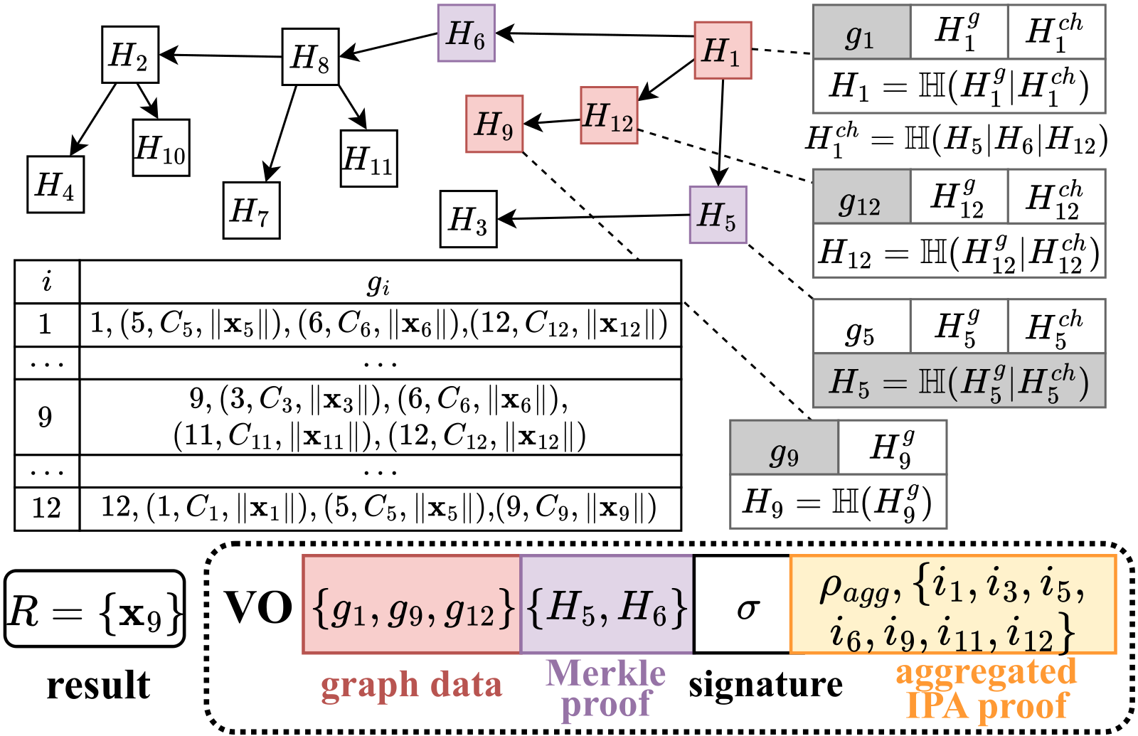
Step 4: what the MeST VO contains. The expanded nodes v1, v12 and v9 each send a record: g1, g12 and g9. g1 holds the commitments and norms of v5, v6 and v12; g12 those of v1, v5 and v9; g9 those of v3, v6, v11 and v12. The other 4 nodes, v3, v5, v6 and v11, all appear in these three records and need no separate proof. The Merkle proof needs only two sibling hashes, H5 and H6, plus the signature, 7 inner products, one merged proof, and the raw vector of the result v9.
Step 5: the client verifies. It computes H9 from g9, then H12 from g12 and H9, then H1 from g1, H5, H6 and H12, and finally adds v1's own commitment and norm to get the root and check the signature. It also checks that v9's raw vector matches v9's commitment. Then it verifies the merged proof, obtains 7 distances, and replays from v1 on the subgraph. The replay reaches v9, matching the cloud's result, and passes. Suppose the cloud cut corners, stopped after expanding v12 and reported v12 as the nearest neighbor. The client replays with the same stopping rule: v9 in the queue is closer than v12, so the search cannot stop yet and must expand v9. Either the VO lacks v9's record or the results don't match, and verification fails either way.
Adding quantization: pruned candidates skip exact authentication
After these two steps, the remaining cost still grows with the number of nodes whose exact distances are computed. Modern ANN systems commonly use quantization to cut exact distance computations. The paper chooses quantization methods like RaBitQ that give a "distance lower bound": if even a candidate's lower bound is farther than the current k-th result, its exact distance is not computed and it is not put in the queue, so it is never expanded.
This kind of pruning suits verification well. The client receives the candidate's quantization code (also authenticated under the signature), computes the lower bound itself when its replay reaches the same point, confirms that it really exceeds the threshold at that moment, and prunes it in the same way, with no need for its exact distance. So only candidates that survive pruning go into the merged proof.
Results
Experiments use six datasets chosen to cover both high dimension and large scale, from the 3,072-dimensional OpenAI3072 (about 1 million vectors) to the 512-dimensional LAION (200 million). Each query uses k = 100, the default bandwidth is 300 Mbps, and the index is HNSW (NSG, another single-layer graph index, on Msmarco, to check that the method does not depend on HNSW). The comparisons are Strawman, ANNProof (which shards the Merkle tree but still sends raw vectors), and their quantized versions. VIDA* is the full version with aggregated IPA plus MeST.
| Setting (OpenAI3072) | Baseline | VIDA family |
|---|---|---|
| Highest recall, end-to-end latency | ANNProof | VIDA* 6.6× faster |
| Highest recall, transmission time | ANNProof | VIDA* 99.2% lower |
| k = 400, latency | ANNProof 6,109 ms, ANNProof-Q 1,506 ms | VIDA*-Q 519 ms |
| 4G bandwidth, latency | ANNProof 16.7 s, ANNProof-Q 3.6 s | VIDA 0.63 s, VIDA-Q 0.82 s |
(Numbers from Section VIII-B of the paper)
The higher the recall target, the larger the advantage. That is because higher recall needs larger HNSW search parameters, more visited nodes, and more vectors for the baselines to send. This shows that what VIDA saves is exactly the transmission that grows with the number of visited nodes.
Bandwidth changes tell the story more clearly. On OpenAI3072, when bandwidth drops from 1,000 Mbps to 40 Mbps, ANNProof's latency rises 11.7 times while VIDA's rises only 1.2 times. When the dimension grows from 512 to 8,192, ANNProof's latency rises 8.5 times and VIDA's 3.9 times. These two sets of numbers show that, within the tested range, VIDA is much less sensitive to bandwidth and dimension than ANNProof.
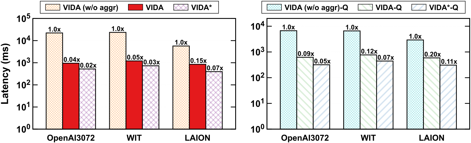
The ablation separates the two optimizations. VIDA (w/o aggr) and VIDA use the same Merkle tree and differ only in whether proofs are merged; merging cuts total latency by 91.9% on average and is 23.3 times faster on OpenAI3072. VIDA* adds MeST on top of VIDA and cuts total latency by another 46.0%. This shows that merging the proofs removes the main bottleneck, and MeST then cuts nearly half of what remains.
What this means for people running vector search services
If you want to add verification to outsourced vector search, don't start by compressing vectors; first ask what the client actually needs to replay the search. VIDA's answer is authenticated distances.
The paper's breakdown suggests an order of checks. First, look at what share of the VO is raw vectors; on high-dimensional embeddings this is usually the largest item. Next, check whether the Merkle proofs are built by node ID; if so, MeST is a reference point: in the paper's experiments it cut total latency by another 46.0% on average, which includes both topology-aware ordering and issuing proofs only for expanded nodes. Quantized pruning can work with this verification as long as the quantization method gives a one-sided lower bound, so the client can recheck each pruning decision.
The cost of the scheme lands on index building. Relative to their baselines, VIDA's index build time is 5.5 times on average and its ADS is 116.1% larger. This is a one-time cost for the data owner, paid for lower query latency and transmission in the paper's main high-dimensional, high-recall settings. Under light workloads it may not pay off: on OpenAI3072 with k of 10 and 25 at low recall targets, VIDA-Q is slower than ANNProof-Q.
Limitations
The scheme applies only to deterministic graph ANN algorithms, since the client must be able to replay the same search step by step. It verifies execution integrity and does not guarantee that the results are the true top-k neighbors.
It does not protect privacy either. The cloud sees the queries and all the data, and the client also receives the result vectors. For settings that need to hide data, the zero-knowledge schemes the paper mentions cost far more; zkRAG, for example, takes about 26 seconds per query to generate a proof.
The experiments simulate the network with toxiproxy rate limiting on a single server, so the latency numbers come from that environment and were not measured on a real cross-cloud deployment.
How did this read for you?
Hoot made a note. Thanks for the feedback.

One tap, no sign-in; tap again to undo. Only anonymous counts are kept, never who you are.
Related papersMore from Paper Daily
 Infra · 2026-11-13Dynamic Graph Indexing for Label-Filtered Approximate Nearest Neighbor SearchVector retrieval often comes with a filter, such as finding nearest neighbors only within a few tags or categories. The hard part is that once a graph index like HNSW is filtered by label, many edges get cut, qualifying points can no longer reach each other, and the search gets stuck locally. DYLAN arranges objects by their label sets in a prefix trie, builds shared graph indices on only some tri…
 Retrieval · 2026-07-24Approximate Nearest Neighbor Search for Modern AI: A Projection-Augmented Graph ApproachDeep dive: Approximate Nearest Neighbor Search for Modern AI: A Projection-Augmented Graph Approach.
 Infra · 2026-10-28Failure-Resilient and Verifiable Distributed Approximate Nearest-Neighbor RetrievalReplicas in a distributed vector database keep results available but do not make them trustworthy. A compromised replica can return validly signed but tampered nearest neighbors. TrustANN adds middleware above the router. For each shard it greedily picks a set of replica replies that meets a set minimum size, scores high on pairwise similarity (candidate overlap plus rank agreement), and spans a…
 Infra · 2026-11-04OctEx: Billion-Scale Vector Search by Precomputed Lattice Neighbor Lists on GPUsFor high-recall vector search on GPUs, graph search is held back by its chain of dependent rounds, not by distance computation itself. OctEx spends GPU memory on neighbor lists precomputed at build time. It makes a few hundred randomly projected low-dimensional copies of the data, cuts each copy into grid cells, and stores for every cell a list of the vectors closest to its center. A query comput…
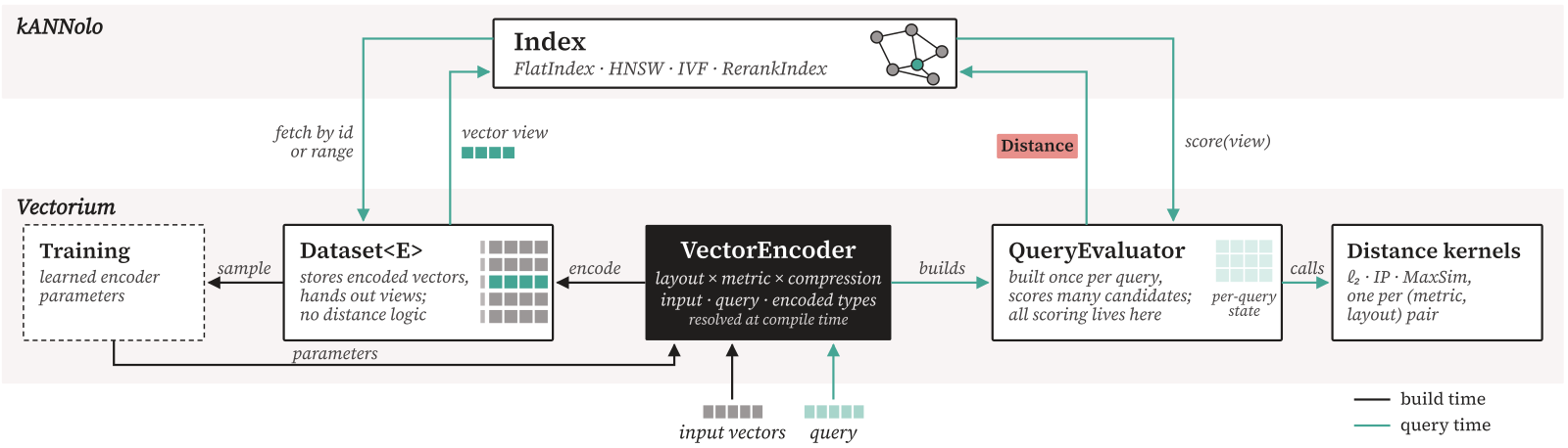 Infra · 2026-11-05Modular and Efficient Approximate Nearest Neighbors Search with Vectorium and kANNoloIn vector search, switching to another embedding form or quantizer often means switching libraries. Existing ANN libraries either support one combination or write separate code for each, and no ANN library covers dense, sparse and multi-vector embeddings behind one interface. The authors release two open-source Rust libraries to fix this: Vectorium stores vectors, computes distances and quantizes…
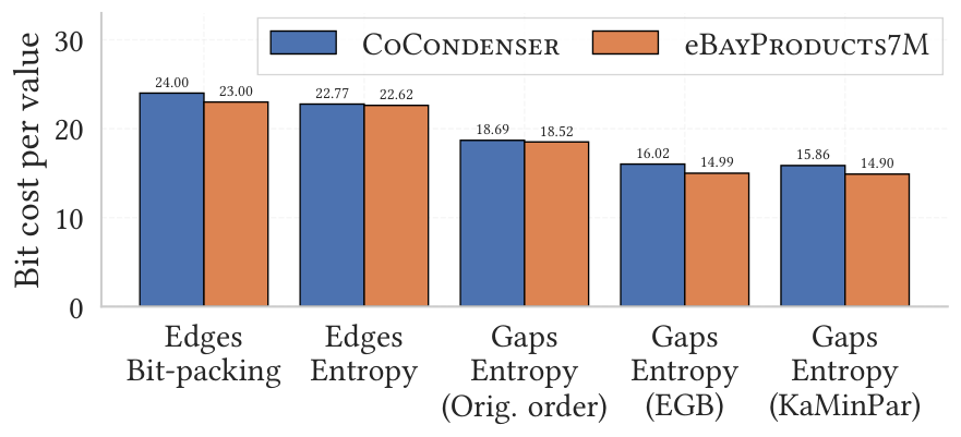 Infra · 2026-10-29Lossless Compression of Proximity Graph Indexes for Efficient Approximate Nearest Neighbors SearchIn HNSW graph indexes for vector search, the vectors are often already quantized, so the edges in the adjacency lists become the main memory cost. Edges are decoded on the fly while each query walks the graph, so compression cannot slow queries down. This work from eBay and the University of Pisa renumbers nodes offline so that neighbors get nearby IDs, then decodes with the SIMD-friendly integer…
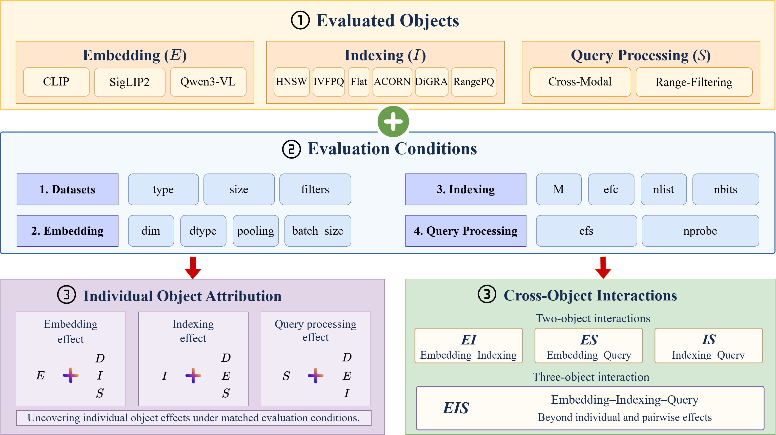 Infra · 2026-11-16VecDBLens: An Evaluatology-Based Framework for Vector Database DiagnosisWhen a vector database recalls poorly, the first instinct is to tune the index, but the ceiling on what an index can find is set by the embedding. On VisualNews with SigLIP2 and exact brute-force search, the authors find that only 2.04% of the nearest images by distance are the paired image in the labels. By contrast, graph indexes such as HNSW and CAGRA keep almost all of exact search's recall.…
Discussion
Add experiment details, reproduction notes or a different take. Requires a GitHub sign-in.
Loading the discussion…