 SIGMOD 2027
Contents · 6 sections
1Label sets arranged in a prefix tree2A region builds its own graph only when it drops to a lower power of 23Queries find non-overlapping regions, then borrow ancestor graphs as bridges4Insertions let a graph grow to 4x before rebuilding5Experiments: a clear lead on label-rich datasets6Where it does not winSHARE

Label-filtered vector search must find the most similar vectors while also meeting a label condition, for example review chunks whose business is both a restaurant and a bar. The difficulty is that label filtering suits inverted lists, while approximate nearest-neighbor search suits graphs such as HNSW. A strict condition cuts the walkable part of the graph into disconnected pieces, and constant inserts quickly make indexes prebuilt per label combination stale. DYLAN (the paper's dynamically updatable index for label-filtered vector search) groups objects that share a label prefix into a region. A region gets its own HNSW graph only once it drops to a lower power of 2; other regions borrow a higher region's graph, and at query time graphs from higher regions also serve as bridges. In single-threaded experiments on 6 real datasets, DYLAN leads most on YTB-Audio: at recall ≥ 0.95, queries that require every query label are 43.5× faster than the fastest baseline. DYLAN's speed comes from this frugal graph-building rule: build a new graph only when a region gets clearly smaller, and borrow the higher graph otherwise. The cost is slower index building than some baselines, and more memory on datasets with many label sets.
The paper's examples come from RAG-style retrieval and multimedia data. A Yelp review chunk has an embedding and also carries the category labels of its business. If a user wants chunks that are closest to a sentence and whose business is both a restaurant and a bar, the system must satisfy a label condition on top of nearest-neighbor search. The paper supports two basic conditions: containment requires an object's label set to include every query label, while overlap only requires one of them. Both can be combined with "and" and "or" into more complex conditions.
The difficulty is that the two requirements favor different data structures. Label filtering suits inverted lists, while approximate nearest neighbor search (ANNS) suits graphs such as HNSW. The stricter the condition, the fewer graph vertices the search may walk through, and the graph breaks into disconnected pieces. Data also keeps arriving, so an index prebuilt for particular label combinations soon goes stale.
We use the six objects from Figure 1 of the paper as a running example (illustrative: a 2D plane, with labels written as numbers).
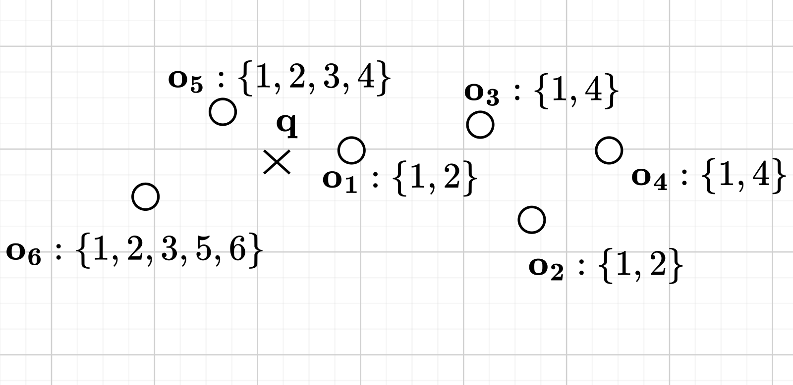
Without a filter, the two objects closest to q are o1 and o5. Under containment {1,3}, the answer becomes o5 and o6, because only they carry both label 1 and label 3. Under overlap {4,5}, the qualifying objects are o3, o4, o5 and o6.
Existing approaches each run into trouble on this example. Filtering first and then scanning is slow when the candidate set is large. Running ANNS first and filtering afterwards needs heavy over-retrieval to keep recall. Filtering while walking a single global HNSW (in-filtering) fails more quietly: in the edges drawn for Root.G in Figure 2 of the paper, the only neighbor of o4 is o2, which carries neither 4 nor 5, so the search never reaches o4. UNG (a label-aware graph index) builds one graph per group of objects with exactly the same label set, so overlap {4,5} lands on three small graphs for {1,4}, {1,2,3,4} and {1,2,3,5,6}. UNG connects related subgraphs with an LNG (label navigating graph), but for queries spanning multiple regions like this one, cross-region connectivity may still be insufficient. A new label set may also trigger widespread changes to the structure between groups.
Label sets arranged in a prefix tree
DYLAN first numbers labels by global frequency, from most to least frequent. Each object's labels are sorted by ascending ID and inserted into a trie (prefix tree), followed by a terminal symbol #. Frequent labels therefore sit near the root, and many objects share the same prefix. The ordering is purely frequency-based and assumes no semantic hierarchy among labels.
Each node of the trie stands for a region: all objects whose label sequence starts with that node's prefix. The trie for our example looks like this (node names follow Figure 2 of the paper; the size level is explained in the next section):
| Node | Prefix | Objects in the region | Size level | Graph used |
|---|---|---|---|---|
| Root | empty | o1–o6, 6 objects | 2 | builds Root.G |
| u1 | {1} | o1–o6, 6 objects | 2 | borrows Root.G |
| u2 | {1,2} | o1, o2, o5, o6 | 2 | borrows Root.G |
| u3 | {1,4} | o3, o4 | 1 | builds u3.G |
| u4 | {1,2,3} | o5, o6 | 1 | builds u4.G |
| u10 | {1,2,#} | o1, o2 | 1 | builds u10.G |
| u5 | {1,2,3,4} | o5 | 0 | builds u5.G |
| u6 | {1,2,3,5} | o6 | 0 | builds u6.G |
This table is the core intermediate product of the DYLAN index. For containment {1,3}, the search only reads the inverted list of label 3 (the larger ID and the rarer of the two), finds u4, and checks that its prefix contains 1. The region of u4 is exactly {o5, o6}, so u4.G holds only qualifying objects and no unqualified vertex blocks the path.
A region builds its own graph only when it drops to a lower power of 2
The simplest idea is to build a graph for every node. The cost is that an object with 50 labels would appear in about 50 graphs along its path. The other extreme is to build only Root.G, which brings back the problem of o4 being unreachable.
DYLAN's compromise assigns each region a size level (the paper calls it log_size): the base-2 logarithm of its object count, rounded down, which says between which two powers of 2 the region falls. Only the root, or a node whose size level is lower than its parent's, builds an HNSW graph on its own region. A node with the same size level as its parent borrows the graph its parent uses.
The table lets us check this rule directly. u2 has 4 objects at size level 2, the same as its parent u1, so it borrows Root.G; the borrowed graph has 6 vertices, within twice 4. u3 has only 2 objects, its size level drops to 1, and it builds its own graph.
With larger numbers (illustrative): a parent region of 1500 objects (size level 10) and a child region of 1000 objects (size level 9), so the child builds its own graph. If the parent has 1000 and the child 600, both lie between 512 and 1023 at size level 9, so the child borrows the parent's graph; the borrowed graph has fewer than 1024 vertices, less than twice 600.
The rule guarantees two things. First, the graph any region uses is at most twice the size of the region, so the number of extra unqualified vertices in it is bounded. Second, the size level can drop at most log2 n times along a root-to-leaf path, so the number of graphs each object enters is on the order of O(min(number of labels, log n)), and the total index size stays near-linear.
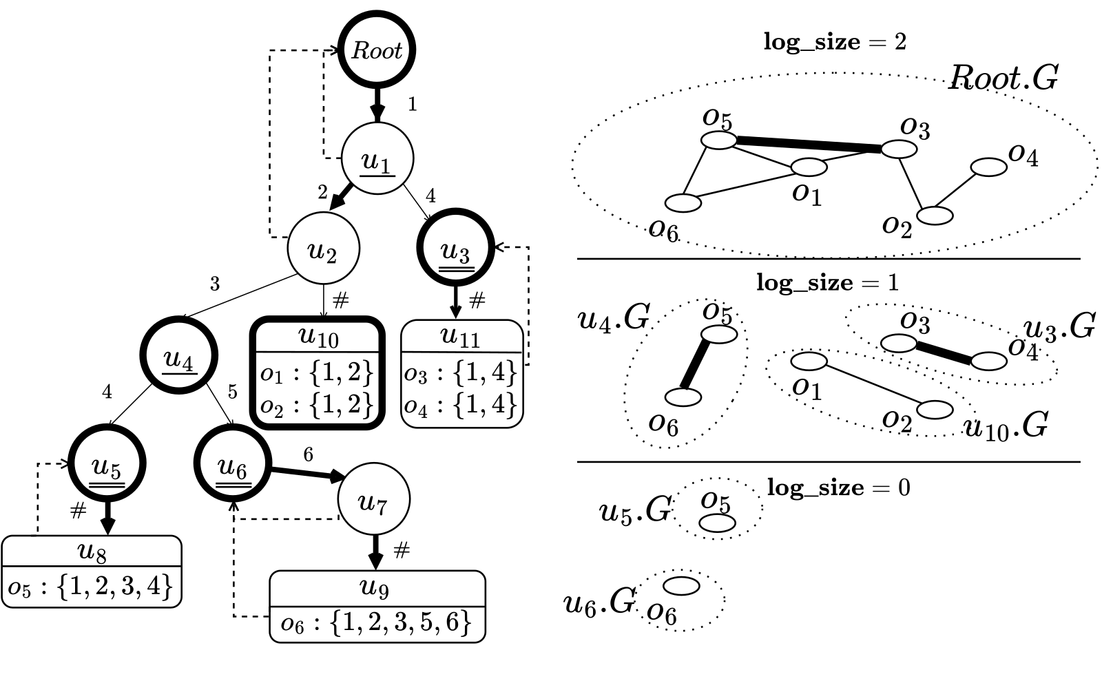
The figure also shows a detail: o5 appears in Root.G, u4.G and u5.G, but its vector is stored only once in a global array, and graph adjacency lists store only object IDs. The authors measured on LAION1M that this extra indirection changes query performance by less than 1%.
Queries find non-overlapping regions, then borrow ancestor graphs as bridges
Containment {1,3} falls into a single region, but overlap {4,5} does not. A query takes three steps; here they are for overlap {4,5}:
| Step | What it does | Output in the example |
|---|---|---|
| 1. Find the cover set | Find regions in the trie that do not overlap and together contain exactly all qualifying objects | {u3, u5, u6}, i.e. {o3,o4}, {o5}, {o6} |
| 2. Add key ancestors | If cover-set nodes appear in two or more child subtrees of a node, add the graph that node uses | u4 and u1 are key ancestors, adding u4.G and Root.G (u1 borrows Root.G) |
| 3. Multi-graph search | Run one joint search over all selected graphs with a shared candidate queue | From o5, walk to o3 via Root.G and to o6 via u4.G |
Step 1 only guarantees that these regions cover all qualifying objects without overlapping, and that the graph each region uses is at most twice the size of the region. The paper gives no guarantee that a region stays connected after filtering; supplementEdges (which gives vertices with too few bottom-layer neighbors extra neighbors sharing the same label) and ancestor bridge edges are the remedies. In the example, o4 is now directly connected to o3 in u3.G and is no longer blocked by o2. Yet u3.G, u5.G and u6.G are isolated from each other; with only these graphs, each graph still has an entry point, but without cross-region links the search may stop early at a local optimum and miss closer candidates in other regions.
Step 2 is meant to ease this. A key ancestor's region contains several cover regions, and its graph is built on the larger object set, so it may already have edges linking different cover regions that can serve as bridges, though connectivity after filtering is not guaranteed. In the example, the edge o5→o3 in Root.G and the edge o5→o6 in u4.G are such bridges.
Step 3 is multi-graph search: when a vertex is expanded, its neighbors in every selected graph are examined. Each neighbor's labels are checked first, and only qualifying neighbors trigger a vector fetch from the global array and a distance computation; once 2M qualifying neighbors are found, expansion of that vertex stops. Why not search each graph separately and merge the results? That cost grows with the number of cover nodes, and the ablation later tests exactly this alternative.
The 2x bound applies only to the graph each region uses, not to the union of all selected graphs. The authors state explicitly that it does not bound the total number of vertices visited by multi-graph search.
Insertions let a graph grow to 4x before rebuilding
Insertions enlarge regions, change size levels, and so change which graph each node borrows. Rebuilding a graph at every change would be too expensive. A new object is first inserted into the trie and then written into the graphs that regions along its root-to-leaf path build themselves; only after that are borrowing relationships adjusted. DYLAN copies or re-borrows first and rebuilds only after the gap passes a threshold.
Illustration: a parent region grows from 1000 to 1024 objects and its size level rises from 9 to 10, while a child region of 600 objects stays at size level 9 and can no longer borrow the parent's graph. DYLAN copies the parent's graph for the child; the copy keeps being used as long as its size level exceeds the child's by at most 1, and is rebuilt on the child's region only when the gap exceeds 1. Conversely, when a region grows to the same size level as its parent, it destroys its own graph and borrows the parent's.
With a gap of at most 1 level, the graph has fewer vertices than 4 times the power of 2 at the region's size level, so the paper proves that the graph each region uses is at most 4 times the region's size; rebuild costs are amortized over later insertions, and the amortized cost per insertion is bounded. Deletions are only marked and skipped during search; under heavy deletion, invalid vertices accumulate and periodic compaction is needed. A new label simply takes the next ID and branches near the leaves, without reordering the whole trie.
Experiments: a clear lead on label-rich datasets
The experiments are single-threaded and fully in memory, on 6 real datasets with roughly 1 million to 5 million vectors and label universes from 29 to 181,931 labels. Every method is tuned for QPS at recall 0.9, and results take the top 10. Among the baselines, Curator is based on IVF clustering, and RWalks encodes labels into the vectors.
On TripClick and LAION1M, which have few labels and simple label sets, DYLAN is 5x faster than the best baseline for containment queries at recall 0.99. This shows that DYLAN loses nothing even when the setting is easy.
The gap is largest on YTB-Audio (YouTube audio, with thousands of machine-generated topical labels). At recall at least 0.8, DYLAN is 5.7x faster than the fastest baseline for containment and 2.3x faster for overlap; at recall at least 0.95, the speedups are 43.5x and 8.7x. This shows that the more fragmented the labels and the higher the recall target, the more the filter breaks the graph apart, and the more the bridge edges are worth.
The authors measured search cost at recall 0.9. On YTB-Audio, DYLAN visits 38.6x fewer points and performs 75.5x fewer distance computations than UNG. The two numbers differ because points rejected by the label filter incur no distance computation. The authors conclude that the speedup comes from the index design rather than implementation-level optimization, which is consistent with checking labels before computing distances and with the bound on unqualified vertices in each region's graph.
In the ablation, replacing multi-graph search with searching each graph separately and merging the results clearly lowers the QPS-recall curve, most visibly for overlap queries on YFCC (Flickr image and video embeddings, with many labels and an uneven label distribution). This shows that, in this experiment, searching the graphs jointly in one search works better than searching each separately and merging.
When an index built on 80% of the data absorbs the remaining 20% by insertion, DYLAN's average insertion time is 3 to 5x faster than that of Filtered-DiskANN, another graph-index baseline. The updated index and an index rebuilt directly on the final data have nearly overlapping recall-QPS curves.
Where it does not win
DYLAN also loses in places. On YTB-Video, any index must access many vectors to reach high recall, and the IVF-based Curator, which incurs less random access, matches DYLAN at high recall. In the selectivity experiments, UNG ties with DYLAN on LAION1M at very low selectivity, and DYLAN is not the best on YFCC at very low selectivity.
The costs are on the books too: index construction is slower than UNG and RWalks, and memory is higher on datasets with many label sets. Of the 2.80GB total index on YFCC, the trie alone takes 1.09GB, because its label universe is large and its label combinations are complex.
Back to the opening rule: label prefixes divide objects into regions, size levels decide which regions deserve their own graph, and ancestor graphs provide bridges between regions. DYLAN's speedup comes mainly from walking fewer unqualified points and computing fewer unnecessary distances.
How did this read for you?
Hoot made a note. Thanks for the feedback.

One tap, no sign-in; tap again to undo. Only anonymous counts are kept, never who you are.
Related papersMore from Paper Daily
 Retrieval · 2026-07-24Approximate Nearest Neighbor Search for Modern AI: A Projection-Augmented Graph ApproachDeep dive: Approximate Nearest Neighbor Search for Modern AI: A Projection-Augmented Graph Approach.
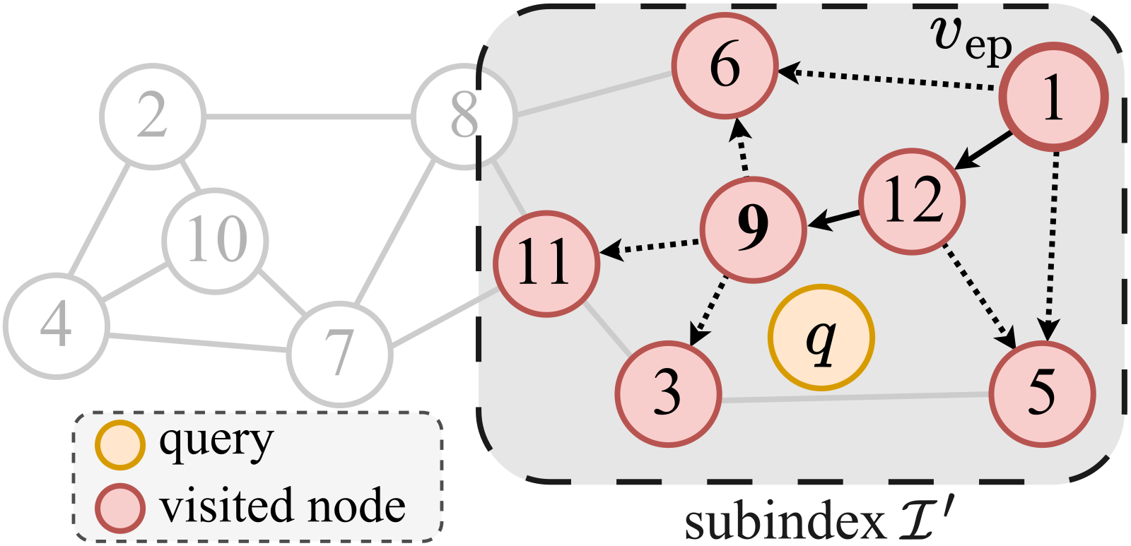 Infra · 2026-11-16Authenticated Approximate Nearest Neighbor Search in Outsourced Vector DatabasesOnce a vector database is outsourced to a third-party cloud, the provider may skip neighbors to save compute or even tamper with results, so the client needs a way to verify that a nearest-neighbor search is genuine. Existing methods have the cloud send back the traversal path on the graph index along with every raw vector visited on the way, and the client recomputes the distances itself. Embedd…
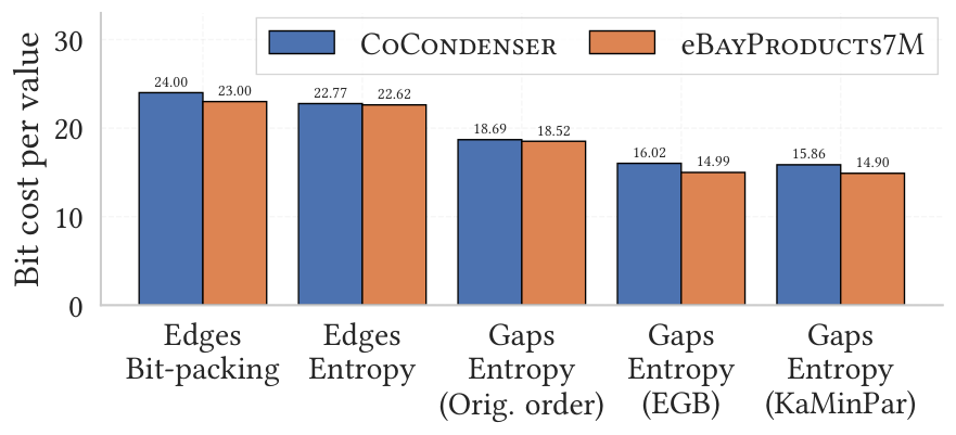 Infra · 2026-10-29Lossless Compression of Proximity Graph Indexes for Efficient Approximate Nearest Neighbors SearchIn HNSW graph indexes for vector search, the vectors are often already quantized, so the edges in the adjacency lists become the main memory cost. Edges are decoded on the fly while each query walks the graph, so compression cannot slow queries down. This work from eBay and the University of Pisa renumbers nodes offline so that neighbors get nearby IDs, then decodes with the SIMD-friendly integer…
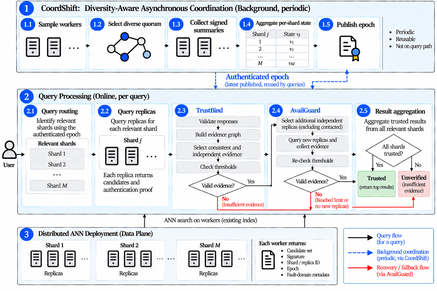 Infra · 2026-10-28Failure-Resilient and Verifiable Distributed Approximate Nearest-Neighbor RetrievalReplicas in a distributed vector database keep results available but do not make them trustworthy. A compromised replica can return validly signed but tampered nearest neighbors. TrustANN adds middleware above the router. For each shard it greedily picks a set of replica replies that meets a set minimum size, scores high on pairwise similarity (candidate overlap plus rank agreement), and spans a…
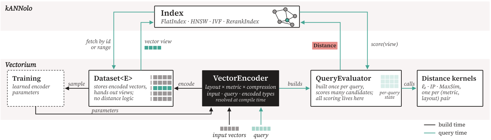 Infra · 2026-11-05Modular and Efficient Approximate Nearest Neighbors Search with Vectorium and kANNoloIn vector search, switching to another embedding form or quantizer often means switching libraries. Existing ANN libraries either support one combination or write separate code for each, and no ANN library covers dense, sparse and multi-vector embeddings behind one interface. The authors release two open-source Rust libraries to fix this: Vectorium stores vectors, computes distances and quantizes…
 Infra · 2026-11-04OctEx: Billion-Scale Vector Search by Precomputed Lattice Neighbor Lists on GPUsFor high-recall vector search on GPUs, graph search is held back by its chain of dependent rounds, not by distance computation itself. OctEx spends GPU memory on neighbor lists precomputed at build time. It makes a few hundred randomly projected low-dimensional copies of the data, cuts each copy into grid cells, and stores for every cell a list of the vectors closest to its center. A query comput…
Discussion
Add experiment details, reproduction notes or a different take. Requires a GitHub sign-in.
Loading the discussion…